[](https://github.com/PlatosTwin/bayes_ab/actions?workflow=Tests)
[](https://codecov.io/gh/PlatosTwin/bayes_ab)
[](https://pypi.org/project/bayes_ab/)
# Bayesian A/B testing
`bayes_ab` is a small package for running Bayesian A/B(/C/D/...) tests.
## Installation
`bayes_ab` can be installed using pip:
```console
pip install bayes_ab
```
Alternatively, you can clone the repository and use `poetry` manually:
```console
cd bayes_ab
pip install poetry
poetry install
poetry shell
```
## Tests and metrics
### Implemented tests
- [BinaryDataTest](https://github.com/PlatosTwin/bayes_ab/blob/main/bayes_ab/experiments/binary.py)
- **_Input data_** — binary (`[0, 1, 0, ...]`)
- Designed for binary data, such as conversions
- [PoissonDataTest](https://github.com/PlatosTwin/bayes_ab/blob/main/bayes_ab/experiments/poisson.py)
- **_Input data_** — integer counts
- Designed for count data (e.g., number of sales per salesman, deaths per zip code)
- [NormalDataTest](https://github.com/PlatosTwin/bayes_ab/blob/main/bayes_ab/experiments/normal.py)
- **_Input data_** — normal data with unknown variance
- Designed for normal data
- [DeltaLognormalDataTest](https://github.com/PlatosTwin/bayes_ab/blob/main/bayes_ab/experiments/delta_lognormal.py)
- **_Input data_** — lognormal data with zeros
- Designed for lognormal data, such as revenue per conversions
- [DiscreteDataTest](https://github.com/PlatosTwin/bayes_ab/blob/main/bayes_ab/experiments/discrete.py)
- **_Input data_** — categorical data with numerical categories
- Designed for discrete data (e.g. dice rolls, star ratings, 1-10 ratings)
### Implemented evaluation metrics
- `Chance to beat all`
- Probability of beating all other variants
- `Expected Loss`
- Risk associated with choosing a given variant over other variants
- Measured in the same units as the tested measure (e.g. positive rate or average value)
- `Uplift vs. 'A'`
- Relative uplift of a given variant compared to the first variant added
- `95% HDI`
- The central interval containing 95% of the probability. The Bayesian approach allows us to say that, 95% of the
time, the 95% HDI will contain the true value
Evaluation metrics are calculated using Monte Carlo simulations from posterior distributions
### Decision rules for test continuation
For tests between two variants with binary, Poisson, and normal data, `bayes_ab` can additionally provide a continuation
recommendation—that is, a recommendation as to the variant to select, or to continue testing.
See the docstrings and examples for usage guidelines.
The decision method makes use of the following concepts:
- **Region of Practical Equivalence (ROPE)** — a region `[-t, t]` of the distribution of differences `B - A` which is
practically equivalent to no uplift. E.g., you may be indifferent between an uplift of +/- 0.1% and no change, in
which case the ROPE would be `[-0.1, 0.1`.
- **95% HDI** — the central interval containing 95% of the probability for the distribution of differences
`B - A`.
The recommendation output has three elements:
1. **Decision**
- Select either variant if the ROPE is fully contained within the 95% HDI.
- Select the better variant if the ROPE and the 95% HDI do not overlap.
- Continue testing if the ROPE partially overlaps the 95% HDI.
- _Note: There are high-confidence and low-confidence variations of the first two messages.
2. **Confidence**
- _High_ if the width of the 95% HDI is less than or equal to `0.8*rope`.
- _Low_ if the width of the 95% HDI is greater than `0.8*rope`.
3. **Bounds**
- The 95% HDI.
### Closed form solutions
For smaller Binary and Poisson samples, metrics calculated from Monte Carlo simulation can be checked against the
closed-form solutions by passing `closed_form=True` to the `evaluate()` method. Larger samples generate warnings;
samples that are larger than a predetermined threshold will raise an error. The larger the sample, however, the closer
the simulated value will be to the true value, so closed-form comparisons are recommended to validate metrics for
smaller samples only.
### Error tolerance
Binary tests with small sample sizes will raise a warning when the error for the expected loss estimate surpasses a set
tolerance. To reduce error, increase the simulation count. For more detail, see the docstring
for `expected_loss_accuracy_bernoulli`
in [`evaluation.py`](https://github.com/PlatosTwin/bayes_ab/blob/main/bayes_ab/metrics/evaluation.py)
## Basic Usage
There are five primary classes:
- `BinaryDataTest`
- `PoissonDataTest`
- `NormalDataTest`
- `DeltaLognormalDataTest`
- `DiscreteDataTest`
For each class, there are two methods for inserting data:
- `add_variant_data` - add raw data for a variant as a list of observations (or numpy 1-D array)
- `add_variant_data_agg` - add aggregated variant data (this can be practical for a larger data set, as the aggregation
can be done outside the package)
Both methods for adding data allow the user to specify a prior distribution (see details in respective docstrings). The
default priors are non-informative priors and should be sufficient for most use cases, and in particular when the number
of samples or observations is large.
To get the results of the test, simply call method `evaluate`; to access evaluation metrics as well as the simulated
random samples, call the `data` instance variable.
Chance to beat all and expected loss are approximated using Monte Carlo simulation, so `evaluate` may return slightly
different values for different runs. To decrease variation, you can set the `sim_count` parameter of `evaluate`
to a higher value (the default is 200K); to fix values, set the `seed` parameter.
More examples are available in the [examples directory](https://github.com/PlatosTwin/bayes_ab/blob/main/examples/),
though many examples in this directory are still in the process of being updated to reflect the functionality of the
updated package.
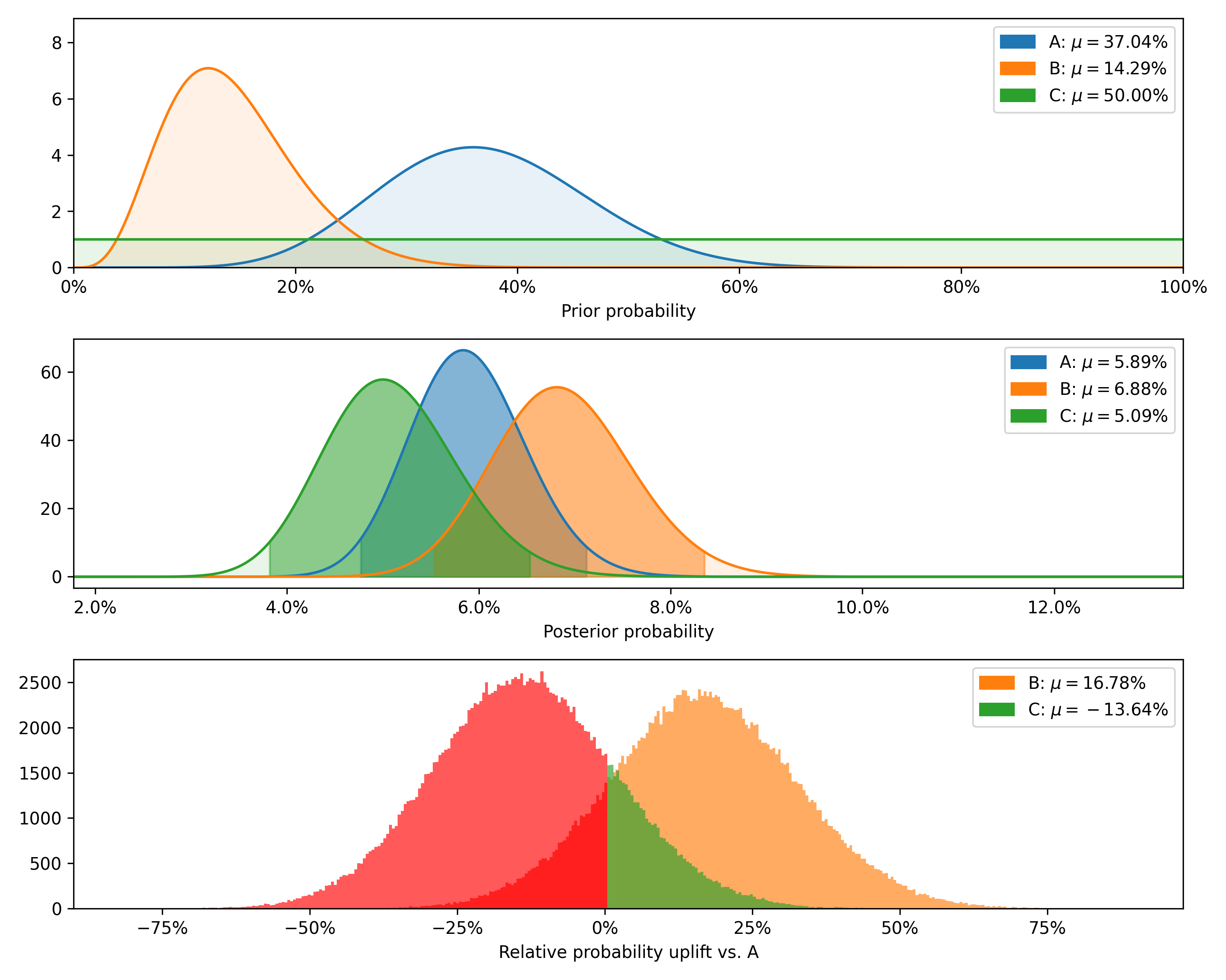
### BinaryDataTest
Class for Bayesian A/B testing of binary-like data (e.g. conversions, successes, etc.).
**Example:**
```python
import numpy as np
from bayes_ab.experiments import BinaryDataTest
# generating some random data
rng = np.random.default_rng(52)
# random 1x1500 array of 0/1 data with 5.2% probability for 1:
data_a = rng.binomial(n=1, p=0.052, size=1500)
# random 1x1200 array of 0/1 data with 6.7% probability for 1:
data_b = rng.binomial(n=1, p=0.067, size=1200)
# initialize a test:
test = BinaryDataTest()
# add variant using raw data (arrays of zeros and ones) and specifying priors:
test.add_variant_data("A", data_a, a_prior=10, b_prior=17)
test.add_variant_data("B", data_b, a_prior=5, b_prior=30)
# the default priors are a=b=1
# test.add_variant_data("C", data_c)
# add variant using aggregated data:
test.add_variant_data_agg("C", total=1000, positives=50)
# evaluate test:
test.evaluate(seed=314)
# access simulation samples and evaluation metrics
data = test.data
# generate plots
test.plot_distributions(control='A', fname='binary_distributions_example.png')
```
+---------+--------+-----------+-------------+----------------+--------------------+---------------+----------------+----------------+
| Variant | Totals | Positives | Sample rate | Posterior rate | Chance to beat all | Expected loss | Uplift vs. "A" | 95% HDI |
+---------+--------+-----------+-------------+----------------+--------------------+---------------+----------------+----------------+
| B | 1200 | 80 | 6.67% | 6.88% | 83.82% | 0.08% | 16.78% | [5.74%, 8.11%] |
| C | 1000 | 50 | 5.00% | 5.09% | 2.54% | 1.87% | -13.64% | [4.00%, 6.28%] |
| A | 1500 | 80 | 5.33% | 5.89% | 13.64% | 1.07% | 0.00% | [4.94%, 6.92%] |
+---------+--------+-----------+-------------+----------------+--------------------+---------------+----------------+----------------+
For smaller samples, such as the above, it is also possible to check the modeled chance to beat all against the
closed-form equivalent by passing `closed_form=True`.
```python
test.evaluate(closed_form=True, seed=314)
```
+---------+-------------------------+--------------------------+--------+
| Variant | Est. chance to beat all | Exact chance to beat all | Delta |
+---------+-------------------------+--------------------------+--------+
| B | 83.82% | 83.58% | 0.28% |
| C | 2.54% | 2.56% | -0.66% |
| A | 13.64% | 13.86% | -1.59% |
+---------+-------------------------+--------------------------+--------+
Removing variant 'C', as this feature is implemented for two variants only currently, and passing a value to `control`
additionally returns a test-continuation recommendation:
```python
test.delete_variant("C")
test.evaluate(control='A', seed=314)
```
Decision: Stop and implement either variant. Confidence: Low. Bounds: [-0.84%, 2.85%].
Finally, we can plot the prior and posterior distributions, as well as the distribution of differences.
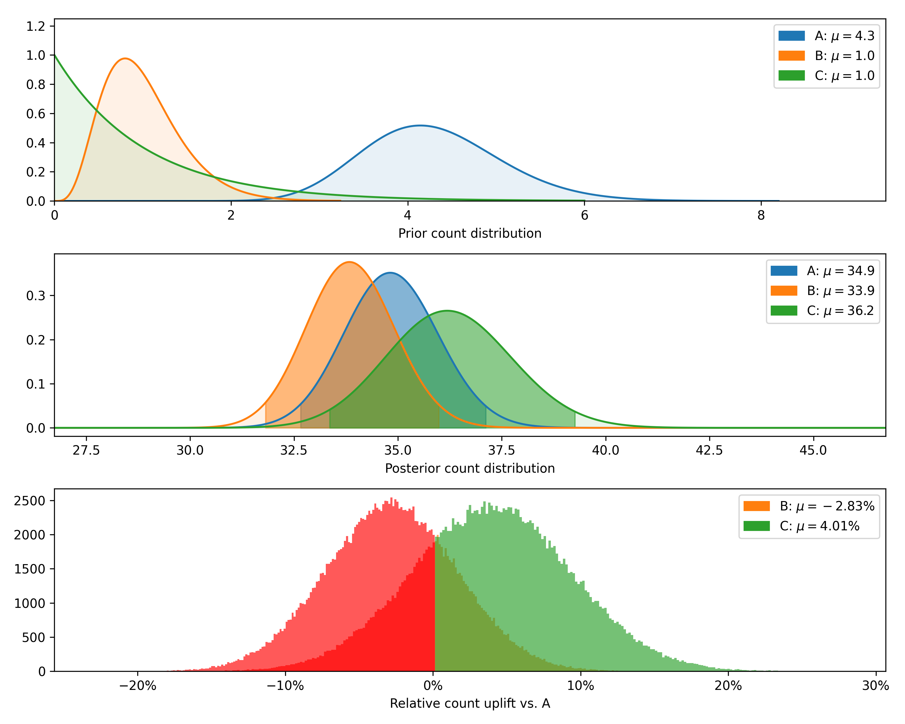
### PoissonDataTest
Class for Bayesian A/B testing of count data. This can be used to compare, e.g., the number of sales per day from
different salesmen, or the number of deaths from a given disease per zip code.
**Example:**
```python
# generating some random data
import numpy as np
from bayes_ab.experiments import PoissonDataTest
# generating some random data
rng = np.random.default_rng(21)
data_a = rng.poisson(43, size=20)
data_b = rng.poisson(39, size=25)
data_c = rng.poisson(37, size=15)
# initialize a test:
test = PoissonDataTest()
# add variant using raw data (arrays of zeros and ones) and specifying priors:
test.add_variant_data("A", data_a, a_prior=30, b_prior=7)
test.add_variant_data("B", data_b, a_prior=5, b_prior=5)
# test.add_variant_data("C", data_c)
# add variant using aggregated data:
test.add_variant_data_agg("C", total=len(data_c), obs_mean=np.mean(data_c), obs_sum=sum(data_c))
# evaluate test:
test.evaluate(seed=314)
# access simulation samples and evaluation metrics
data = test.data
# generate plots
test.plot_distributions(control='A', fname='poisson_distributions_example.png')
```
+---------+--------------+-------------+----------------+--------------------+---------------+----------------+--------------+
| Variant | Observations | Sample mean | Posterior mean | Chance to beat all | Expected loss | Uplift vs. "A" | 95% HDI |
+---------+--------------+-------------+----------------+--------------------+---------------+----------------+--------------+
| C | 15 | 38.6 | 36.2 | 74.06% | 0.28 | 4.01% | [33.8, 38.8] |
| B | 25 | 40.4 | 33.9 | 5.09% | 2.66 | -2.83% | [32.1, 35.6] |
| A | 20 | 45.6 | 34.9 | 20.85% | 1.68 | 0.00% | [33.0, 36.7] |
+---------+--------------+-------------+----------------+--------------------+---------------+----------------+--------------+
For samples smaller than the above, it is also possible to check the modeled chance to beat all against the closed-form
equivalent by passing `closed_form=True`:
```python
test.evaluate(closed_form=True, seed=314)
```
+---------+-------------------------+--------------------------+--------+
| Variant | Est. chance to beat all | Exact chance to beat all | Delta |
+---------+-------------------------+--------------------------+--------+
| C | 74.06% | 73.91% | 0.20% |
| B | 5.09% | 5.24% | -2.84% |
| A | 20.85% | 20.85% | -0.01% |
+---------+-------------------------+--------------------------+--------+
Removing variant 'C', as this feature is implemented for two variants only currently, and passing `control` and `rope`
additionally returns a test-continuation recommendation:
```python
test.delete_variant("C")
test.evaluate(control='A', rope=0.5, seed=314)
```
Decision: Stop and implement either variant. Confidence: Low. Bounds: [-4.0, 2.1].
Finally, we can plot the posterior distributions as well as the distribution of differences (returning now to the
original number of observations rather than the smaller sample used to show the closed-form validation).
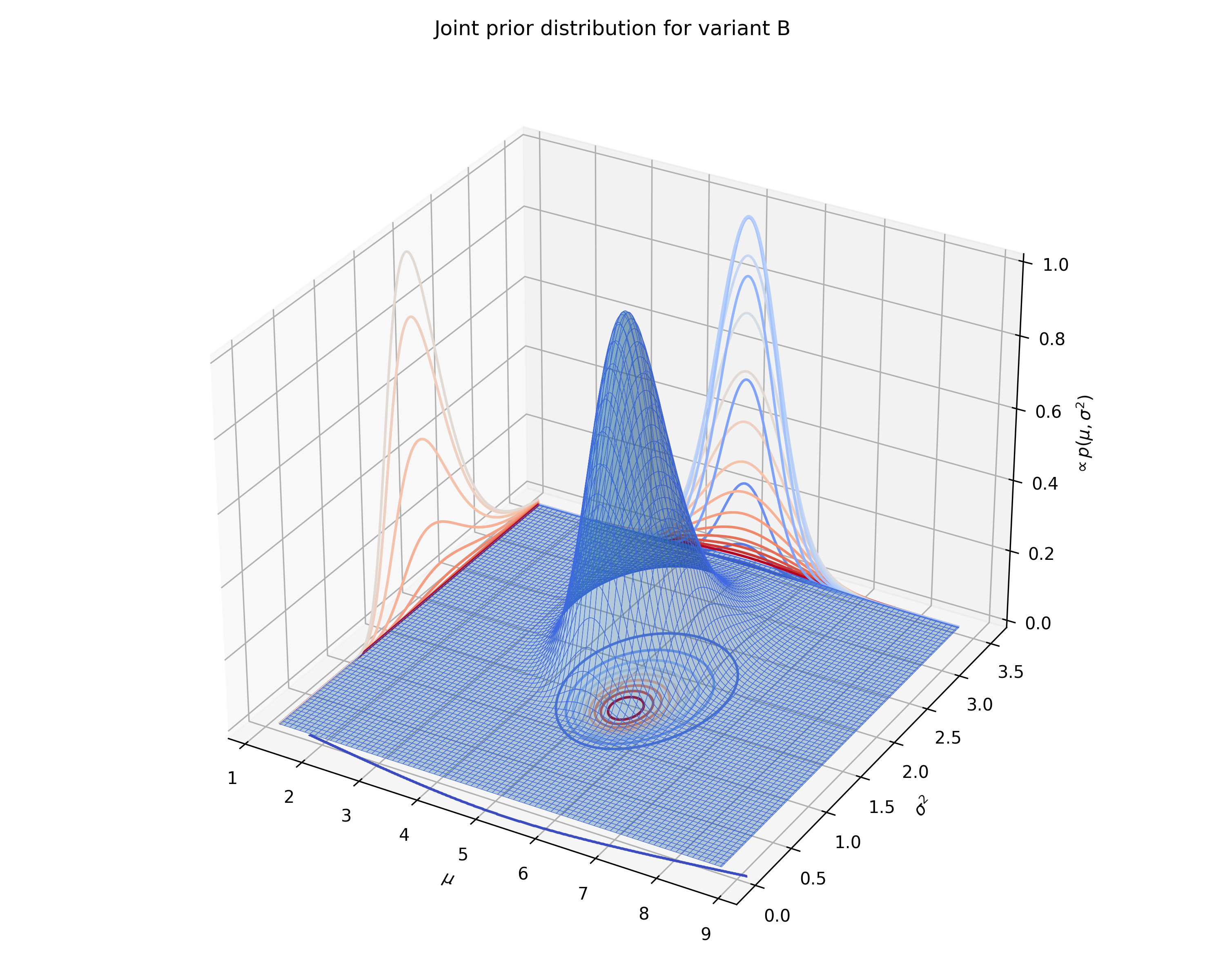
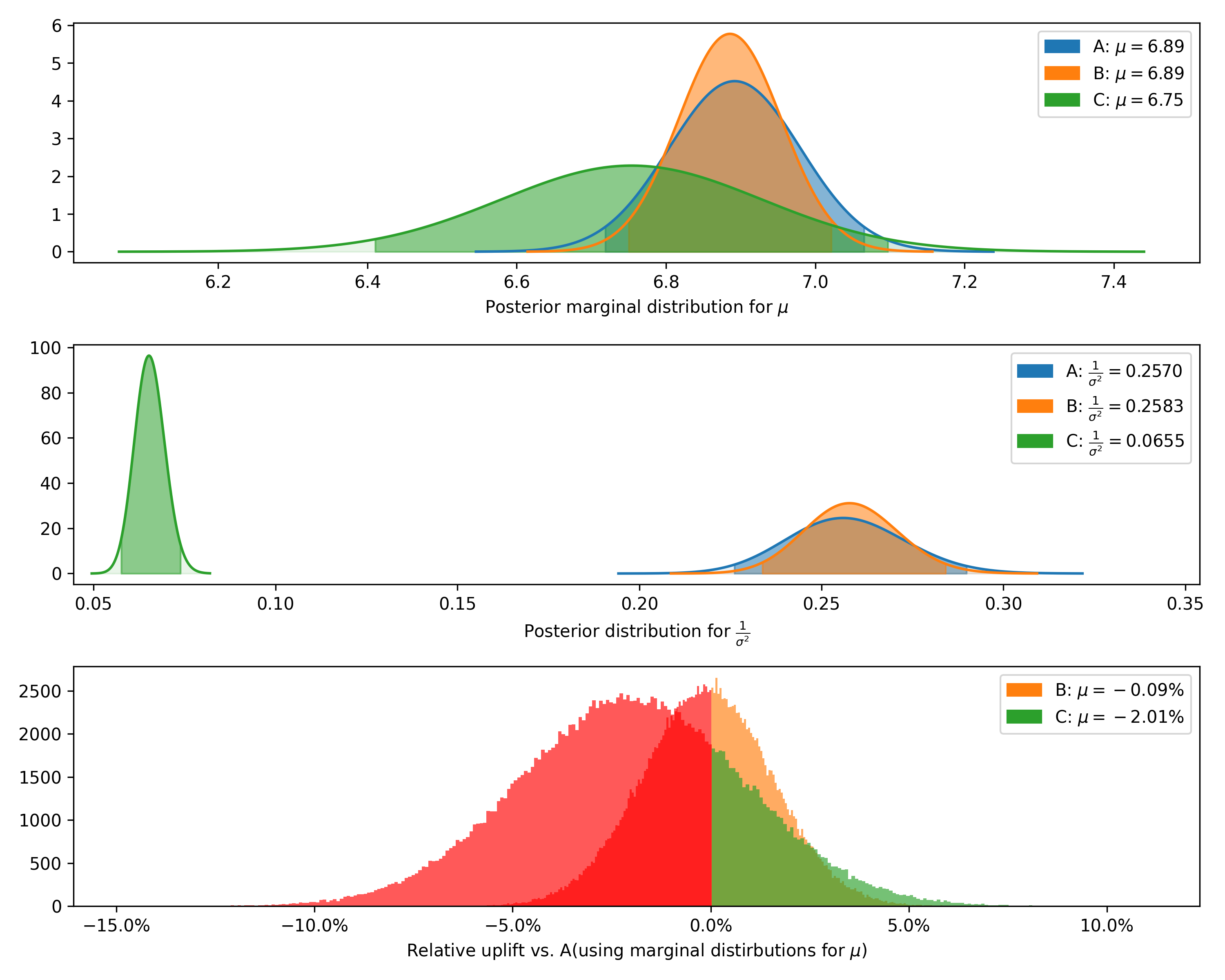
### NormalDataTest
Class for Bayesian A/B test for normal data.
**Example:**
```python
import numpy as np
from bayes_ab.experiments import NormalDataTest
# generating some random data
rng = np.random.default_rng(314)
data_a = rng.normal(6.9, 2, 500)
data_b = rng.normal(6.89, 2, 800)
data_c = rng.normal(7.0, 4, 500)
# initialize a test:
test = NormalDataTest()
# add variant using raw data:
test.add_variant_data("A", data_a)
test.add_variant_data("B", data_b, m_prior=5, n_prior=11, v_prior=10, s_2_prior=4)
# test.add_variant_data("C", data_c)
# add variant using aggregated data:
test.add_variant_data_agg("C", len(data_c), sum(data_c), sum((data_c - np.mean(data_c)) ** 2), sum(np.square(data_c)))
# evaluate test:
test.evaluate(sim_count=200000, seed=314)
# access simulation samples and evaluation metrics
data = test.data
# generate plots
test.plot_joint_prior(variant='B', fname='normal_prior_distribution_B_example.png')
test.plot_distributions(control='A', fname='normal_distributions_example.png')
```
+---------+--------------+-------------+----------------+-----------+-----------+--------------------+---------------+----------------+----------------+-----------------+
| Variant | Observations | Sample mean | Posterior mean | Precision | Std. dev. | Chance to beat all | Expected loss | Uplift vs. "A" | 95% HDI (mean) | 95% HDI (stdev) |
+---------+--------------+-------------+----------------+-----------+-----------+--------------------+---------------+----------------+----------------+-----------------+
| A | 500 | 6.89 | 6.89 | 0.257 | 1.97 | 91.31% | 0.0 | 0.00% | [6.72, 7.07] | [1.86, 2.10] |
| B | 800 | 6.91 | 6.89 | 0.258 | 1.97 | 8.69% | 0.01 | -0.09% | [6.75, 7.02] | [1.88, 2.07] |
| C | 500 | 6.75 | 6.75 | 0.065 | 3.91 | 0.00% | 0.14 | -2.01% | [6.41, 7.10] | [3.68, 4.17] |
+---------+--------------+-------------+----------------+-----------+-----------+--------------------+---------------+----------------+----------------+-----------------+
We can also plot the joint prior distribution for $\mu$ and $\sigma^2$, the posterior distributions for $\mu$ and
$\frac{1}{\sigma^2}$, and the distribution of differences from a given control.
### DeltaLognormalDataTest
Class for Bayesian A/B testing of delta-lognormal data (log-normal with zeros). Delta-lognormal data is typical case of
revenue per session data where many sessions have 0 revenue but non-zero values are positive numbers with possible
log-normal distribution. To handle this data, the calculation is combining binary Bayes model for zero vs non-zero
"conversions" and log-normal model for non-zero values.
**Example:**
```python
import numpy as np
from bayes_ab.experiments import DeltaLognormalDataTest
test = DeltaLognormalDataTest()
data_a = [7.1, 0.3, 5.9, 0, 1.3, 0.3, 0, 1.2, 0, 3.6, 0, 1.5, 2.2, 0, 4.9, 0, 0, 1.1, 0, 0, 7.1, 0, 6.9, 0]
data_b = [4.0, 0, 3.3, 19.3, 18.5, 0, 0, 0, 12.9, 0, 0, 0, 10.2, 0, 0, 23.1, 0, 3.7, 0, 0, 11.3, 10.0, 0, 18.3, 12.1]
# adding variant using raw data:
test.add_variant_data("A", data_a)
# test.add_variant_data("B", data_b)
# alternatively, variant can be also added using aggregated data:
# (looks more complicated but for large data it can be quite handy to move around only these sums)
test.add_variant_data_agg(
name="B",
total=len(data_b),
positives=sum(x > 0 for x in data_b),
sum_values=sum(data_b),
sum_logs=sum([np.log(x) for x in data_b if x > 0]),
sum_logs_2=sum([np.square(np.log(x)) for x in data_b if x > 0])
)
# evaluate test:
test.evaluate(seed=21)
# access simulation samples and evaluation metrics
data = test.data
```
[{'variant': 'A',
'totals': 24,
'positives': 13,
'sum_values': 43.4,
'avg_values': 1.80833,
'avg_positive_values': 3.33846,
'prob_being_best': 0.04815,
'expected_loss': 4.0941101},
{'variant': 'B',
'totals': 25,
'positives': 12,
'sum_values': 146.7,
'avg_values': 5.868,
'avg_positive_values': 12.225,
'prob_being_best': 0.95185,
'expected_loss': 0.1588627}]
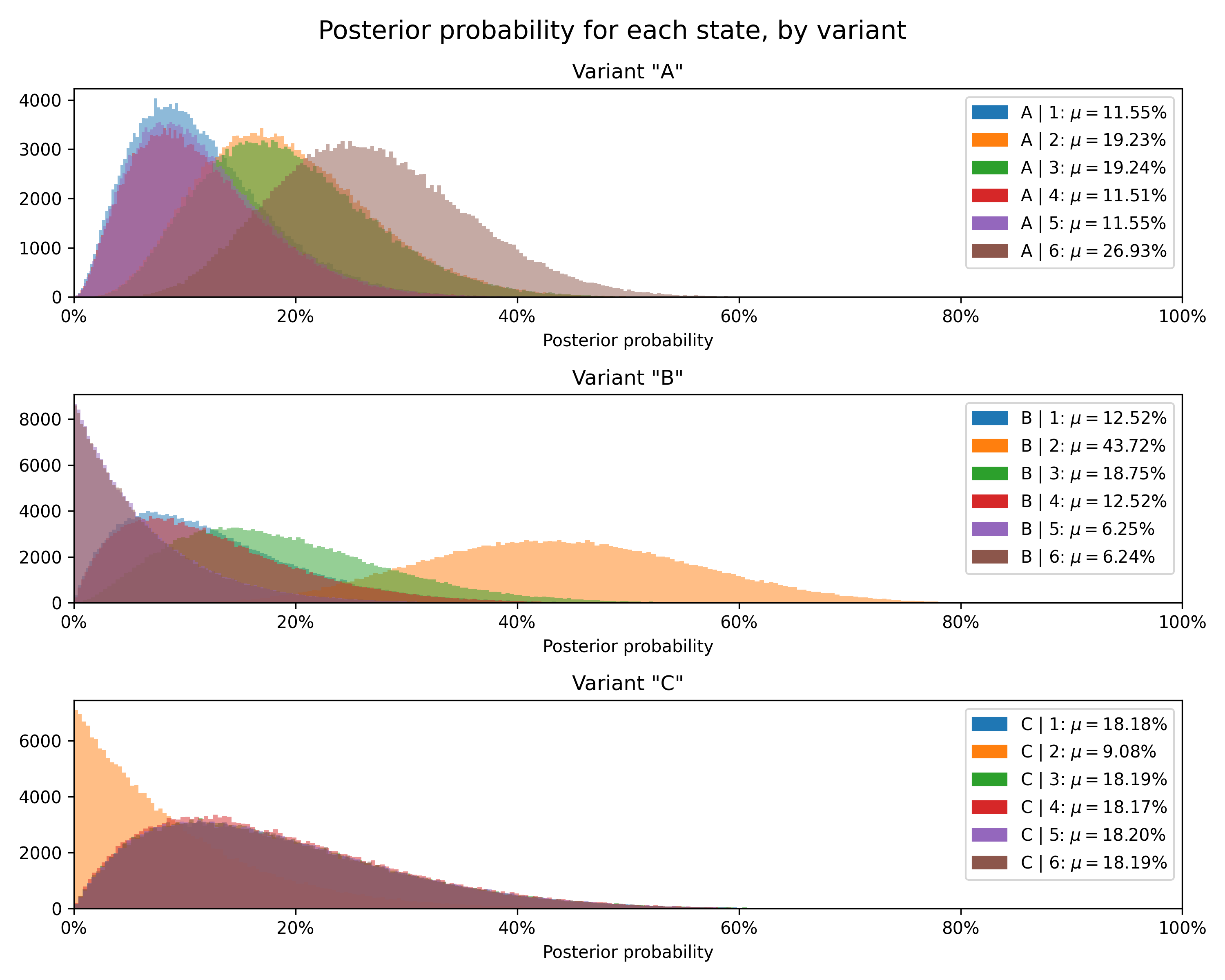
### DiscreteDataTest
Class for Bayesian A/B testing for discrete data having a finite number of numerical categories (states).
This test can be used, e.g., to find the biases of different dice and to decide which of them of multiple for the "best"
of multiple dice) or rating
data
(e.g. 1-5 stars or 1-10 scale).
**Example:**
```python
from bayes_ab.experiments import DiscreteDataTest
# dice rolls data for 3 dice - A, B, C
data_a = [2, 5, 1, 4, 6, 2, 2, 6, 3, 2, 6, 3, 4, 6, 3, 1, 6, 3, 5, 6]
data_b = [1, 2, 2, 2, 2, 3, 2, 3, 4, 2]
data_c = [1, 3, 6, 5, 4]
# initialize a test with all possible states (i.e. numerical categories):
test = DiscreteDataTest(states=[1, 2, 3, 4, 5, 6])
# add variant using raw data:
test.add_variant_data("A", data_a)
test.add_variant_data("B", data_b)
test.add_variant_data("C", data_c)
# add variant using aggregated data:
# test.add_variant_data_agg("C", [1, 0, 1, 1, 1, 1]) # equivalent to rolls in data_c
# evaluate test:
test.evaluate(sim_count=200000, seed=52)
# access simulation samples and evaluation metrics
data = test.data
```
+---------+------------------------------------+-------------+----------------+------------------------------------------------------------------+-------------------------------------------------------------------------------------------------------------------------+--------------------+---------------+----------------+----------------+
| Variant | Concentrations | Sample mean | Posterior mean | Relative prob. | 95% HDI (relative prob.) | Chance to beat all | Expected loss | Uplift vs. "A" | 95% HDI (mean) |
+---------+------------------------------------+-------------+----------------+------------------------------------------------------------------+-------------------------------------------------------------------------------------------------------------------------+--------------------+---------------+----------------+----------------+
| A | 1: 2, 2: 4, 3: 4, 4: 2, 5: 2, 6: 6 | 3.8 | 3.73 | 1: 11.54%, 2: 19.23%, 3: 19.23%, 4: 11.54%, 5: 11.54%, 6: 26.92% | 1: [2.55%, 26.02%], 2: [6.82%, 36.06%], 3: [6.85%, 36.12%], 4: [2.54%, 25.96%], 5: [2.59%, 26.09%], 6: [12.10%, 45.17%] | 55.21% | 19.71% | 0.00% | [3.07, 4.40] |
| C | 1: 1, 2: 0, 3: 1, 4: 1, 5: 1, 6: 1 | 3.8 | 3.64 | 1: 18.18%, 2: 9.09%, 3: 18.18%, 4: 18.18%, 5: 18.18%, 6: 18.18% | 1: [2.50%, 44.45%], 2: [0.26%, 30.78%], 3: [2.51%, 44.54%], 4: [2.47%, 44.48%], 5: [2.53%, 44.57%], 6: [2.52%, 44.54%] | 44.02% | 29.09% | -2.53% | [2.64, 4.58] |
| B | 1: 1, 2: 6, 3: 2, 4: 1, 5: 0, 6: 0 | 2.3 | 2.75 | 1: 12.50%, 2: 43.75%, 3: 18.75%, 4: 12.50%, 5: 6.25%, 6: 6.25% | 1: [1.66%, 31.97%], 2: [21.33%, 67.67%], 3: [4.31%, 40.47%], 4: [1.65%, 31.96%], 5: [0.17%, 21.78%], 6: [0.17%, 21.84%] | 0.78% | 117.81% | -26.29% | [2.18, 3.45] |
+---------+------------------------------------+-------------+----------------+------------------------------------------------------------------+-------------------------------------------------------------------------------------------------------------------------+--------------------+---------------+----------------+----------------+
Finally, we can plot the posterior distribution for each state for each variant.
## Development
To set up a development environment, use [Poetry](https://python-poetry.org/) and [pre-commit](https://pre-commit.com):
```console
pip install poetry
poetry install
poetry run pre-commit install
```
## Roadmap
Improvements in the pipeline:
- Validate and improve `DeltaLognormalDataTest`
- Add test continuation assessment (decision, confidence, bounds)
- Create formatted output
- Add plotting for posteriors and differences from control
- Update Jupyter examples folder
- Implement sample size/reverse posterior calculation
- Create a method to easily plot evolutions of posteriors and evaluation metrics with time
- Annotate classes with references to the relevant sections within Gelman et al., 2021
- Implement Markov Chain Monte Carlo in place of Monte Carlo, using `pymc`
## References and related work
The development of this package has relied on the resources outlined below. Where a function or method draws directly on
a particular derivation, the docstring contains the exact reference.
- [Bayesian A/B Testing at VWO](https://vwo.com/downloads/VWO_SmartStats_technical_whitepaper.pdf)
(Chris Stucchio, 2015)
- [Optional stopping in data collection: p values, Bayes factors, credible intervals, precision](
http://doingbayesiandataanalysis.blogspot.com/2013/11/optional-stopping-in-data-collection-p.html)
(John Kruschke, 2013)
- [Is Bayesian A/B Testing Immune to Peeking? Not Exactly](http://varianceexplained.org/r/bayesian-ab-testing/)
(David Robinson, 2015)
- [Formulas for Bayesian A/B Testing](https://www.evanmiller.org/bayesian-ab-testing.html) (Evan Miller, 2015)
- [Easy Evaluation of Decision Rules in Bayesian A/B testing](
https://www.chrisstucchio.com/blog/2014/bayesian_ab_decision_rule.html) (Chris Stucchio, 2014)
- _[Bayesian Data Analysis, Third Edition](http://www.stat.columbia.edu/~gelman/book/BDA3.pdf)_ (Gelman et al., 2021)
- [Bayesian Inference 2019](https://vioshyvo.github.io/Bayesian_inference/index.html) (Hyvönen & Tolonen, 2019)
- [An Introduction to Bayesian Thinking](https://statswithr.github.io/book/) (Clyde et al., 2022)
There is a wealth of material on Bayesian statistics available freely online. A small and somewhat random selection is
catalogued below.
- [Probabalistic programming and Bayesian methods for hackers](https://nbviewer.org/github/CamDavidsonPilon/Probabilistic-Programming-and-Bayesian-Methods-for-Hackers/tree/master/) (
Cameron Davidson-Pilon, 2022)
- [Think Bayes 2](https://allendowney.github.io/ThinkBayes2/index.html) (Downey, 2021)
- [Continuous Monitoring of A/B Tests without Pain: Optional Stopping in Bayesian Testing](https://arxiv.org/pdf/1602.05549.pdf)
(Deng, Lu, & Chen, 2016)
The dataset `tapwater.csv` is downloaded from the [`statsr`](https://github.com/StatsWithR/statsr/tree/master/data)
repository.
This project was inspired by Aubrey Clayton's (2022) _[Bernoulli's Fallacy:
Statistical Illogic and the Crisis of Modern Science](http://cup.columbia.edu/book/bernoullis-fallacy/9780231199940)_.
## Select online calculators
- [Yanir Seroussi's calculator](https://yanirs.github.io/tools/split-test-calculator/) |
[project description](https://yanirseroussi.com/2016/06/19/making-bayesian-ab-testing-more-accessible/)
- [Lyst's calculator](https://making.lyst.com/bayesian-calculator/)
| [project descrption](https://making.lyst.com/2014/05/10/bayesian-ab-testing/)
- [Dynamic Yield's calculator](https://marketing.dynamicyield.com/bayesian-calculator/)
## A note on forking
This package was forked from Matus Baniar's [`bayesian-testing`](https://github.com/Matt52/bayesian-testing). Upon
deciding to take package development in a different direction, I detached the fork from the original repository. The
original author's contributions are large, however, with his central contributions being to the development of the core
infrastructure of the project. This being the first package I have worked on, the original author's work to prepare this
code for packaging has also been instrumental to package publication, not to mention educative.
Raw data
{
"_id": null,
"home_page": "https://github.com/PlatosTwin/bayes_ab",
"name": "bayes-ab",
"maintainer": "",
"docs_url": null,
"requires_python": ">=3.8,<4.0",
"maintainer_email": "",
"keywords": "ab testing,bayes,bayesian statistics",
"author": "Nikita Bogdanov",
"author_email": "",
"download_url": "https://files.pythonhosted.org/packages/4f/2b/a3a207133bc368e5657499e649fe9d82a609f5b497d466062e0ead16303f/bayes_ab-0.4.3.tar.gz",
"platform": null,
"description": "[](https://github.com/PlatosTwin/bayes_ab/actions?workflow=Tests)\n[](https://codecov.io/gh/PlatosTwin/bayes_ab)\n[](https://pypi.org/project/bayes_ab/)\n\n# Bayesian A/B testing\n\n`bayes_ab` is a small package for running Bayesian A/B(/C/D/...) tests.\n\n## Installation\n\n`bayes_ab` can be installed using pip:\n\n```console\npip install bayes_ab\n```\n\nAlternatively, you can clone the repository and use `poetry` manually:\n\n```console\ncd bayes_ab\npip install poetry\npoetry install\npoetry shell\n```\n\n## Tests and metrics\n\n### Implemented tests\n\n- [BinaryDataTest](https://github.com/PlatosTwin/bayes_ab/blob/main/bayes_ab/experiments/binary.py)\n - **_Input data_** \u2014 binary (`[0, 1, 0, ...]`)\n - Designed for binary data, such as conversions\n- [PoissonDataTest](https://github.com/PlatosTwin/bayes_ab/blob/main/bayes_ab/experiments/poisson.py)\n - **_Input data_** \u2014 integer counts\n - Designed for count data (e.g., number of sales per salesman, deaths per zip code)\n- [NormalDataTest](https://github.com/PlatosTwin/bayes_ab/blob/main/bayes_ab/experiments/normal.py)\n - **_Input data_** \u2014 normal data with unknown variance\n - Designed for normal data\n- [DeltaLognormalDataTest](https://github.com/PlatosTwin/bayes_ab/blob/main/bayes_ab/experiments/delta_lognormal.py)\n - **_Input data_** \u2014 lognormal data with zeros\n - Designed for lognormal data, such as revenue per conversions\n- [DiscreteDataTest](https://github.com/PlatosTwin/bayes_ab/blob/main/bayes_ab/experiments/discrete.py)\n - **_Input data_** \u2014 categorical data with numerical categories\n - Designed for discrete data (e.g. dice rolls, star ratings, 1-10 ratings)\n\n### Implemented evaluation metrics\n\n- `Chance to beat all`\n - Probability of beating all other variants\n- `Expected Loss`\n - Risk associated with choosing a given variant over other variants\n - Measured in the same units as the tested measure (e.g. positive rate or average value)\n- `Uplift vs. 'A'`\n - Relative uplift of a given variant compared to the first variant added\n- `95% HDI`\n - The central interval containing 95% of the probability. The Bayesian approach allows us to say that, 95% of the\n time, the 95% HDI will contain the true value\n\nEvaluation metrics are calculated using Monte Carlo simulations from posterior distributions\n\n### Decision rules for test continuation\n\nFor tests between two variants with binary, Poisson, and normal data, `bayes_ab` can additionally provide a continuation\nrecommendation\u2014that is, a recommendation as to the variant to select, or to continue testing.\nSee the docstrings and examples for usage guidelines.\n\nThe decision method makes use of the following concepts:\n\n- **Region of Practical Equivalence (ROPE)** \u2014 a region `[-t, t]` of the distribution of differences `B - A` which is\n practically equivalent to no uplift. E.g., you may be indifferent between an uplift of +/- 0.1% and no change, in\n which case the ROPE would be `[-0.1, 0.1`.\n- **95% HDI** \u2014 the central interval containing 95% of the probability for the distribution of differences\n `B - A`.\n\nThe recommendation output has three elements:\n\n1. **Decision**\n - Select either variant if the ROPE is fully contained within the 95% HDI.\n - Select the better variant if the ROPE and the 95% HDI do not overlap.\n - Continue testing if the ROPE partially overlaps the 95% HDI.\n - _Note: There are high-confidence and low-confidence variations of the first two messages.\n2. **Confidence**\n - _High_ if the width of the 95% HDI is less than or equal to `0.8*rope`.\n - _Low_ if the width of the 95% HDI is greater than `0.8*rope`.\n3. **Bounds**\n - The 95% HDI.\n\n### Closed form solutions\n\nFor smaller Binary and Poisson samples, metrics calculated from Monte Carlo simulation can be checked against the\nclosed-form solutions by passing `closed_form=True` to the `evaluate()` method. Larger samples generate warnings;\nsamples that are larger than a predetermined threshold will raise an error. The larger the sample, however, the closer\nthe simulated value will be to the true value, so closed-form comparisons are recommended to validate metrics for\nsmaller samples only.\n\n### Error tolerance\n\nBinary tests with small sample sizes will raise a warning when the error for the expected loss estimate surpasses a set\ntolerance. To reduce error, increase the simulation count. For more detail, see the docstring\nfor `expected_loss_accuracy_bernoulli`\nin [`evaluation.py`](https://github.com/PlatosTwin/bayes_ab/blob/main/bayes_ab/metrics/evaluation.py)\n\n## Basic Usage\n\nThere are five primary classes:\n\n- `BinaryDataTest`\n- `PoissonDataTest`\n- `NormalDataTest`\n- `DeltaLognormalDataTest`\n- `DiscreteDataTest`\n\nFor each class, there are two methods for inserting data:\n\n- `add_variant_data` - add raw data for a variant as a list of observations (or numpy 1-D array)\n- `add_variant_data_agg` - add aggregated variant data (this can be practical for a larger data set, as the aggregation\n can be done outside the package)\n\nBoth methods for adding data allow the user to specify a prior distribution (see details in respective docstrings). The\ndefault priors are non-informative priors and should be sufficient for most use cases, and in particular when the number\nof samples or observations is large.\n\nTo get the results of the test, simply call method `evaluate`; to access evaluation metrics as well as the simulated\nrandom samples, call the `data` instance variable.\n\nChance to beat all and expected loss are approximated using Monte Carlo simulation, so `evaluate` may return slightly\ndifferent values for different runs. To decrease variation, you can set the `sim_count` parameter of `evaluate`\nto a higher value (the default is 200K); to fix values, set the `seed` parameter.\n\nMore examples are available in the [examples directory](https://github.com/PlatosTwin/bayes_ab/blob/main/examples/),\nthough many examples in this directory are still in the process of being updated to reflect the functionality of the\nupdated package.\n\n### BinaryDataTest\n\nClass for Bayesian A/B testing of binary-like data (e.g. conversions, successes, etc.).\n\n**Example:**\n\n```python\nimport numpy as np\nfrom bayes_ab.experiments import BinaryDataTest\n\n# generating some random data\nrng = np.random.default_rng(52)\n# random 1x1500 array of 0/1 data with 5.2% probability for 1:\ndata_a = rng.binomial(n=1, p=0.052, size=1500)\n# random 1x1200 array of 0/1 data with 6.7% probability for 1:\ndata_b = rng.binomial(n=1, p=0.067, size=1200)\n\n# initialize a test:\ntest = BinaryDataTest()\n\n# add variant using raw data (arrays of zeros and ones) and specifying priors:\ntest.add_variant_data(\"A\", data_a, a_prior=10, b_prior=17)\ntest.add_variant_data(\"B\", data_b, a_prior=5, b_prior=30)\n# the default priors are a=b=1\n# test.add_variant_data(\"C\", data_c)\n\n# add variant using aggregated data:\ntest.add_variant_data_agg(\"C\", total=1000, positives=50)\n\n# evaluate test:\ntest.evaluate(seed=314)\n\n# access simulation samples and evaluation metrics\ndata = test.data\n\n# generate plots\ntest.plot_distributions(control='A', fname='binary_distributions_example.png')\n```\n\n +---------+--------+-----------+-------------+----------------+--------------------+---------------+----------------+----------------+\n | Variant | Totals | Positives | Sample rate | Posterior rate | Chance to beat all | Expected loss | Uplift vs. \"A\" | 95% HDI |\n +---------+--------+-----------+-------------+----------------+--------------------+---------------+----------------+----------------+\n | B | 1200 | 80 | 6.67% | 6.88% | 83.82% | 0.08% | 16.78% | [5.74%, 8.11%] |\n | C | 1000 | 50 | 5.00% | 5.09% | 2.54% | 1.87% | -13.64% | [4.00%, 6.28%] |\n | A | 1500 | 80 | 5.33% | 5.89% | 13.64% | 1.07% | 0.00% | [4.94%, 6.92%] |\n +---------+--------+-----------+-------------+----------------+--------------------+---------------+----------------+----------------+\n\nFor smaller samples, such as the above, it is also possible to check the modeled chance to beat all against the\nclosed-form equivalent by passing `closed_form=True`.\n\n```python\ntest.evaluate(closed_form=True, seed=314)\n```\n\n +---------+-------------------------+--------------------------+--------+\n | Variant | Est. chance to beat all | Exact chance to beat all | Delta |\n +---------+-------------------------+--------------------------+--------+\n | B | 83.82% | 83.58% | 0.28% |\n | C | 2.54% | 2.56% | -0.66% |\n | A | 13.64% | 13.86% | -1.59% |\n +---------+-------------------------+--------------------------+--------+\n\nRemoving variant 'C', as this feature is implemented for two variants only currently, and passing a value to `control`\nadditionally returns a test-continuation recommendation:\n\n```python\ntest.delete_variant(\"C\")\ntest.evaluate(control='A', seed=314)\n```\n\n Decision: Stop and implement either variant. Confidence: Low. Bounds: [-0.84%, 2.85%].\n\nFinally, we can plot the prior and posterior distributions, as well as the distribution of differences.\n\n\n\n### PoissonDataTest\n\nClass for Bayesian A/B testing of count data. This can be used to compare, e.g., the number of sales per day from\ndifferent salesmen, or the number of deaths from a given disease per zip code.\n\n**Example:**\n\n```python\n# generating some random data\nimport numpy as np\nfrom bayes_ab.experiments import PoissonDataTest\n\n# generating some random data\nrng = np.random.default_rng(21)\ndata_a = rng.poisson(43, size=20)\ndata_b = rng.poisson(39, size=25)\ndata_c = rng.poisson(37, size=15)\n\n# initialize a test:\ntest = PoissonDataTest()\n\n# add variant using raw data (arrays of zeros and ones) and specifying priors:\ntest.add_variant_data(\"A\", data_a, a_prior=30, b_prior=7)\ntest.add_variant_data(\"B\", data_b, a_prior=5, b_prior=5)\n# test.add_variant_data(\"C\", data_c)\n\n# add variant using aggregated data:\ntest.add_variant_data_agg(\"C\", total=len(data_c), obs_mean=np.mean(data_c), obs_sum=sum(data_c))\n\n# evaluate test:\ntest.evaluate(seed=314)\n\n# access simulation samples and evaluation metrics\ndata = test.data\n\n# generate plots\ntest.plot_distributions(control='A', fname='poisson_distributions_example.png')\n```\n\n +---------+--------------+-------------+----------------+--------------------+---------------+----------------+--------------+\n | Variant | Observations | Sample mean | Posterior mean | Chance to beat all | Expected loss | Uplift vs. \"A\" | 95% HDI |\n +---------+--------------+-------------+----------------+--------------------+---------------+----------------+--------------+\n | C | 15 | 38.6 | 36.2 | 74.06% | 0.28 | 4.01% | [33.8, 38.8] |\n | B | 25 | 40.4 | 33.9 | 5.09% | 2.66 | -2.83% | [32.1, 35.6] |\n | A | 20 | 45.6 | 34.9 | 20.85% | 1.68 | 0.00% | [33.0, 36.7] |\n +---------+--------------+-------------+----------------+--------------------+---------------+----------------+--------------+\n\nFor samples smaller than the above, it is also possible to check the modeled chance to beat all against the closed-form\nequivalent by passing `closed_form=True`:\n\n```python\ntest.evaluate(closed_form=True, seed=314)\n```\n\n +---------+-------------------------+--------------------------+--------+\n | Variant | Est. chance to beat all | Exact chance to beat all | Delta |\n +---------+-------------------------+--------------------------+--------+\n | C | 74.06% | 73.91% | 0.20% |\n | B | 5.09% | 5.24% | -2.84% |\n | A | 20.85% | 20.85% | -0.01% |\n +---------+-------------------------+--------------------------+--------+\n\nRemoving variant 'C', as this feature is implemented for two variants only currently, and passing `control` and `rope`\nadditionally returns a test-continuation recommendation:\n\n```python\ntest.delete_variant(\"C\")\ntest.evaluate(control='A', rope=0.5, seed=314)\n```\n\n Decision: Stop and implement either variant. Confidence: Low. Bounds: [-4.0, 2.1].\n\nFinally, we can plot the posterior distributions as well as the distribution of differences (returning now to the\noriginal number of observations rather than the smaller sample used to show the closed-form validation).\n\n\n\n### NormalDataTest\n\nClass for Bayesian A/B test for normal data.\n\n**Example:**\n\n```python\nimport numpy as np\nfrom bayes_ab.experiments import NormalDataTest\n\n# generating some random data\nrng = np.random.default_rng(314)\ndata_a = rng.normal(6.9, 2, 500)\ndata_b = rng.normal(6.89, 2, 800)\ndata_c = rng.normal(7.0, 4, 500)\n\n# initialize a test:\ntest = NormalDataTest()\n\n# add variant using raw data:\ntest.add_variant_data(\"A\", data_a)\ntest.add_variant_data(\"B\", data_b, m_prior=5, n_prior=11, v_prior=10, s_2_prior=4)\n# test.add_variant_data(\"C\", data_c)\n\n# add variant using aggregated data:\ntest.add_variant_data_agg(\"C\", len(data_c), sum(data_c), sum((data_c - np.mean(data_c)) ** 2), sum(np.square(data_c)))\n\n# evaluate test:\ntest.evaluate(sim_count=200000, seed=314)\n\n# access simulation samples and evaluation metrics\ndata = test.data\n\n# generate plots\ntest.plot_joint_prior(variant='B', fname='normal_prior_distribution_B_example.png')\ntest.plot_distributions(control='A', fname='normal_distributions_example.png')\n```\n\n +---------+--------------+-------------+----------------+-----------+-----------+--------------------+---------------+----------------+----------------+-----------------+\n | Variant | Observations | Sample mean | Posterior mean | Precision | Std. dev. | Chance to beat all | Expected loss | Uplift vs. \"A\" | 95% HDI (mean) | 95% HDI (stdev) |\n +---------+--------------+-------------+----------------+-----------+-----------+--------------------+---------------+----------------+----------------+-----------------+\n | A | 500 | 6.89 | 6.89 | 0.257 | 1.97 | 91.31% | 0.0 | 0.00% | [6.72, 7.07] | [1.86, 2.10] |\n | B | 800 | 6.91 | 6.89 | 0.258 | 1.97 | 8.69% | 0.01 | -0.09% | [6.75, 7.02] | [1.88, 2.07] |\n | C | 500 | 6.75 | 6.75 | 0.065 | 3.91 | 0.00% | 0.14 | -2.01% | [6.41, 7.10] | [3.68, 4.17] |\n +---------+--------------+-------------+----------------+-----------+-----------+--------------------+---------------+----------------+----------------+-----------------+\n\nWe can also plot the joint prior distribution for $\\mu$ and $\\sigma^2$, the posterior distributions for $\\mu$ and\n$\\frac{1}{\\sigma^2}$, and the distribution of differences from a given control.\n\n\n\n\n### DeltaLognormalDataTest\n\nClass for Bayesian A/B testing of delta-lognormal data (log-normal with zeros). Delta-lognormal data is typical case of\nrevenue per session data where many sessions have 0 revenue but non-zero values are positive numbers with possible\nlog-normal distribution. To handle this data, the calculation is combining binary Bayes model for zero vs non-zero\n\"conversions\" and log-normal model for non-zero values.\n\n**Example:**\n\n```python\nimport numpy as np\nfrom bayes_ab.experiments import DeltaLognormalDataTest\n\ntest = DeltaLognormalDataTest()\n\ndata_a = [7.1, 0.3, 5.9, 0, 1.3, 0.3, 0, 1.2, 0, 3.6, 0, 1.5, 2.2, 0, 4.9, 0, 0, 1.1, 0, 0, 7.1, 0, 6.9, 0]\ndata_b = [4.0, 0, 3.3, 19.3, 18.5, 0, 0, 0, 12.9, 0, 0, 0, 10.2, 0, 0, 23.1, 0, 3.7, 0, 0, 11.3, 10.0, 0, 18.3, 12.1]\n\n# adding variant using raw data:\ntest.add_variant_data(\"A\", data_a)\n# test.add_variant_data(\"B\", data_b)\n\n# alternatively, variant can be also added using aggregated data:\n# (looks more complicated but for large data it can be quite handy to move around only these sums)\ntest.add_variant_data_agg(\n name=\"B\",\n total=len(data_b),\n positives=sum(x > 0 for x in data_b),\n sum_values=sum(data_b),\n sum_logs=sum([np.log(x) for x in data_b if x > 0]),\n sum_logs_2=sum([np.square(np.log(x)) for x in data_b if x > 0])\n)\n\n# evaluate test:\ntest.evaluate(seed=21)\n\n# access simulation samples and evaluation metrics\ndata = test.data\n```\n\n [{'variant': 'A',\n 'totals': 24,\n 'positives': 13,\n 'sum_values': 43.4,\n 'avg_values': 1.80833,\n 'avg_positive_values': 3.33846,\n 'prob_being_best': 0.04815,\n 'expected_loss': 4.0941101},\n {'variant': 'B',\n 'totals': 25,\n 'positives': 12,\n 'sum_values': 146.7,\n 'avg_values': 5.868,\n 'avg_positive_values': 12.225,\n 'prob_being_best': 0.95185,\n 'expected_loss': 0.1588627}]\n\n### DiscreteDataTest\n\nClass for Bayesian A/B testing for discrete data having a finite number of numerical categories (states).\nThis test can be used, e.g., to find the biases of different dice and to decide which of them of multiple for the \"best\"\nof multiple dice) or rating\ndata\n(e.g. 1-5 stars or 1-10 scale).\n\n**Example:**\n\n```python\nfrom bayes_ab.experiments import DiscreteDataTest\n\n# dice rolls data for 3 dice - A, B, C\ndata_a = [2, 5, 1, 4, 6, 2, 2, 6, 3, 2, 6, 3, 4, 6, 3, 1, 6, 3, 5, 6]\ndata_b = [1, 2, 2, 2, 2, 3, 2, 3, 4, 2]\ndata_c = [1, 3, 6, 5, 4]\n\n# initialize a test with all possible states (i.e. numerical categories):\ntest = DiscreteDataTest(states=[1, 2, 3, 4, 5, 6])\n\n# add variant using raw data:\ntest.add_variant_data(\"A\", data_a)\ntest.add_variant_data(\"B\", data_b)\ntest.add_variant_data(\"C\", data_c)\n\n# add variant using aggregated data:\n# test.add_variant_data_agg(\"C\", [1, 0, 1, 1, 1, 1]) # equivalent to rolls in data_c\n\n# evaluate test:\ntest.evaluate(sim_count=200000, seed=52)\n\n# access simulation samples and evaluation metrics\ndata = test.data\n```\n\n +---------+------------------------------------+-------------+----------------+------------------------------------------------------------------+-------------------------------------------------------------------------------------------------------------------------+--------------------+---------------+----------------+----------------+\n | Variant | Concentrations | Sample mean | Posterior mean | Relative prob. | 95% HDI (relative prob.) | Chance to beat all | Expected loss | Uplift vs. \"A\" | 95% HDI (mean) |\n +---------+------------------------------------+-------------+----------------+------------------------------------------------------------------+-------------------------------------------------------------------------------------------------------------------------+--------------------+---------------+----------------+----------------+\n | A | 1: 2, 2: 4, 3: 4, 4: 2, 5: 2, 6: 6 | 3.8 | 3.73 | 1: 11.54%, 2: 19.23%, 3: 19.23%, 4: 11.54%, 5: 11.54%, 6: 26.92% | 1: [2.55%, 26.02%], 2: [6.82%, 36.06%], 3: [6.85%, 36.12%], 4: [2.54%, 25.96%], 5: [2.59%, 26.09%], 6: [12.10%, 45.17%] | 55.21% | 19.71% | 0.00% | [3.07, 4.40] |\n | C | 1: 1, 2: 0, 3: 1, 4: 1, 5: 1, 6: 1 | 3.8 | 3.64 | 1: 18.18%, 2: 9.09%, 3: 18.18%, 4: 18.18%, 5: 18.18%, 6: 18.18% | 1: [2.50%, 44.45%], 2: [0.26%, 30.78%], 3: [2.51%, 44.54%], 4: [2.47%, 44.48%], 5: [2.53%, 44.57%], 6: [2.52%, 44.54%] | 44.02% | 29.09% | -2.53% | [2.64, 4.58] |\n | B | 1: 1, 2: 6, 3: 2, 4: 1, 5: 0, 6: 0 | 2.3 | 2.75 | 1: 12.50%, 2: 43.75%, 3: 18.75%, 4: 12.50%, 5: 6.25%, 6: 6.25% | 1: [1.66%, 31.97%], 2: [21.33%, 67.67%], 3: [4.31%, 40.47%], 4: [1.65%, 31.96%], 5: [0.17%, 21.78%], 6: [0.17%, 21.84%] | 0.78% | 117.81% | -26.29% | [2.18, 3.45] |\n +---------+------------------------------------+-------------+----------------+------------------------------------------------------------------+-------------------------------------------------------------------------------------------------------------------------+--------------------+---------------+----------------+----------------+\n\nFinally, we can plot the posterior distribution for each state for each variant.\n\n\n\n## Development\n\nTo set up a development environment, use [Poetry](https://python-poetry.org/) and [pre-commit](https://pre-commit.com):\n\n```console\npip install poetry\npoetry install\npoetry run pre-commit install\n```\n\n## Roadmap\n\nImprovements in the pipeline:\n\n- Validate and improve `DeltaLognormalDataTest`\n - Add test continuation assessment (decision, confidence, bounds)\n - Create formatted output\n - Add plotting for posteriors and differences from control\n- Update Jupyter examples folder\n- Implement sample size/reverse posterior calculation\n- Create a method to easily plot evolutions of posteriors and evaluation metrics with time\n- Annotate classes with references to the relevant sections within Gelman et al., 2021\n- Implement Markov Chain Monte Carlo in place of Monte Carlo, using `pymc`\n\n## References and related work\n\nThe development of this package has relied on the resources outlined below. Where a function or method draws directly on\na particular derivation, the docstring contains the exact reference.\n\n- [Bayesian A/B Testing at VWO](https://vwo.com/downloads/VWO_SmartStats_technical_whitepaper.pdf)\n (Chris Stucchio, 2015)\n- [Optional stopping in data collection: p values, Bayes factors, credible intervals, precision](\n http://doingbayesiandataanalysis.blogspot.com/2013/11/optional-stopping-in-data-collection-p.html)\n (John Kruschke, 2013)\n- [Is Bayesian A/B Testing Immune to Peeking? Not Exactly](http://varianceexplained.org/r/bayesian-ab-testing/)\n (David Robinson, 2015)\n- [Formulas for Bayesian A/B Testing](https://www.evanmiller.org/bayesian-ab-testing.html) (Evan Miller, 2015)\n- [Easy Evaluation of Decision Rules in Bayesian A/B testing](\n https://www.chrisstucchio.com/blog/2014/bayesian_ab_decision_rule.html) (Chris Stucchio, 2014)\n- _[Bayesian Data Analysis, Third Edition](http://www.stat.columbia.edu/~gelman/book/BDA3.pdf)_ (Gelman et al., 2021)\n- [Bayesian Inference 2019](https://vioshyvo.github.io/Bayesian_inference/index.html) (Hyv\u00f6nen & Tolonen, 2019)\n- [An Introduction to Bayesian Thinking](https://statswithr.github.io/book/) (Clyde et al., 2022)\n\nThere is a wealth of material on Bayesian statistics available freely online. A small and somewhat random selection is\ncatalogued below.\n\n- [Probabalistic programming and Bayesian methods for hackers](https://nbviewer.org/github/CamDavidsonPilon/Probabilistic-Programming-and-Bayesian-Methods-for-Hackers/tree/master/) (\n Cameron Davidson-Pilon, 2022)\n- [Think Bayes 2](https://allendowney.github.io/ThinkBayes2/index.html) (Downey, 2021)\n- [Continuous Monitoring of A/B Tests without Pain: Optional Stopping in Bayesian Testing](https://arxiv.org/pdf/1602.05549.pdf)\n (Deng, Lu, & Chen, 2016)\n\nThe dataset `tapwater.csv` is downloaded from the [`statsr`](https://github.com/StatsWithR/statsr/tree/master/data)\nrepository.\n\nThis project was inspired by Aubrey Clayton's (2022) _[Bernoulli's Fallacy:\nStatistical Illogic and the Crisis of Modern Science](http://cup.columbia.edu/book/bernoullis-fallacy/9780231199940)_.\n\n## Select online calculators\n\n- [Yanir Seroussi's calculator](https://yanirs.github.io/tools/split-test-calculator/) |\n [project description](https://yanirseroussi.com/2016/06/19/making-bayesian-ab-testing-more-accessible/)\n- [Lyst's calculator](https://making.lyst.com/bayesian-calculator/)\n | [project descrption](https://making.lyst.com/2014/05/10/bayesian-ab-testing/)\n- [Dynamic Yield's calculator](https://marketing.dynamicyield.com/bayesian-calculator/)\n\n## A note on forking\n\nThis package was forked from Matus Baniar's [`bayesian-testing`](https://github.com/Matt52/bayesian-testing). Upon\ndeciding to take package development in a different direction, I detached the fork from the original repository. The\noriginal author's contributions are large, however, with his central contributions being to the development of the core\ninfrastructure of the project. This being the first package I have worked on, the original author's work to prepare this\ncode for packaging has also been instrumental to package publication, not to mention educative.\n",
"bugtrack_url": null,
"license": "MIT",
"summary": "Bayesian A/B testing.",
"version": "0.4.3",
"split_keywords": [
"ab testing",
"bayes",
"bayesian statistics"
],
"urls": [
{
"comment_text": "",
"digests": {
"md5": "e97dbd7881ebcb761249093ff7da2d30",
"sha256": "15d9afe3ec1304b81ed31c602d1961c551995a77a6858926198af28e17722046"
},
"downloads": -1,
"filename": "bayes_ab-0.4.3-py3-none-any.whl",
"has_sig": false,
"md5_digest": "e97dbd7881ebcb761249093ff7da2d30",
"packagetype": "bdist_wheel",
"python_version": "py3",
"requires_python": ">=3.8,<4.0",
"size": 45980,
"upload_time": "2022-12-19T02:42:15",
"upload_time_iso_8601": "2022-12-19T02:42:15.156966Z",
"url": "https://files.pythonhosted.org/packages/cf/97/2b4f0be27ff32105d42830dc89e58ef8ca4b3f02b099de1a8bfa42c44f86/bayes_ab-0.4.3-py3-none-any.whl",
"yanked": false,
"yanked_reason": null
},
{
"comment_text": "",
"digests": {
"md5": "4771c18e95827b8b934a86d569071cd7",
"sha256": "2fc9b75c47c35ea5373b4e0e2dfefe15ec837225a7591ce80e54bbe67897a18a"
},
"downloads": -1,
"filename": "bayes_ab-0.4.3.tar.gz",
"has_sig": false,
"md5_digest": "4771c18e95827b8b934a86d569071cd7",
"packagetype": "sdist",
"python_version": "source",
"requires_python": ">=3.8,<4.0",
"size": 42791,
"upload_time": "2022-12-19T02:42:16",
"upload_time_iso_8601": "2022-12-19T02:42:16.567614Z",
"url": "https://files.pythonhosted.org/packages/4f/2b/a3a207133bc368e5657499e649fe9d82a609f5b497d466062e0ead16303f/bayes_ab-0.4.3.tar.gz",
"yanked": false,
"yanked_reason": null
}
],
"upload_time": "2022-12-19 02:42:16",
"github": true,
"gitlab": false,
"bitbucket": false,
"github_user": "PlatosTwin",
"github_project": "bayes_ab",
"travis_ci": false,
"coveralls": false,
"github_actions": true,
"lcname": "bayes-ab"
}

