# cvmcore


## Introduction
The core function of data analysis for plot or data process used by SZQ lab from China Agricultural University
## Example usage
```python
from Bio import Phylo
import matplotlib as mpl
import matplotlib.pyplot as plt
from io import StringIO
import matplotlib.collections as mpcollections
from copy import copy
import pandas as pd
import numpy as np
import seaborn as sn
from cvmcore.cvmcore import cvmplot
from scipy.cluster.hierarchy import linkage, dendrogram, complete, to_tree
from scipy.spatial.distance import squareform
```
```python
mlst = [[np.nan, 19., 12., 9., 5., 9., 2.],
[np.nan, 19., 12., 9., 5., 9., 2.],
[10., 17., 12., 9., np.nan, 9., 2.],
[10., 19., 12., np.nan, 5., 9., 2.],
[np.nan, 19., 13., 9., 5., 9., 2.]]
genes = np.char.replace(np.array(np.arange(1, 8), dtype='str'), '', 'gene_', count=1)
samples = np.char.replace(np.array(np.arange(1, 6), dtype='str'), '', 'sample_', count=1)
df_mlst = pd.DataFrame(mlst, index=samples, columns=genes)
diff_matrix = cvmplot.get_diff_df(df_mlst)
```
```python
diff_matrix
```
<div>
<table border="1" class="dataframe">
<thead>
<tr style="text-align: right;">
<th></th>
<th>sample_1</th>
<th>sample_2</th>
<th>sample_3</th>
<th>sample_4</th>
<th>sample_5</th>
</tr>
</thead>
<tbody>
<tr>
<th>sample_1</th>
<td>0</td>
<td>0</td>
<td>1</td>
<td>0</td>
<td>1</td>
</tr>
<tr>
<th>sample_2</th>
<td>0</td>
<td>0</td>
<td>1</td>
<td>0</td>
<td>1</td>
</tr>
<tr>
<th>sample_3</th>
<td>1</td>
<td>1</td>
<td>0</td>
<td>1</td>
<td>2</td>
</tr>
<tr>
<th>sample_4</th>
<td>0</td>
<td>0</td>
<td>1</td>
<td>0</td>
<td>1</td>
</tr>
<tr>
<th>sample_5</th>
<td>1</td>
<td>1</td>
<td>2</td>
<td>1</td>
<td>0</td>
</tr>
</tbody>
</table>
</div>
```python
link_matrix =linkage(squareform(diff_matrix), method='complete')
```
```python
link_matrix
```
array([[0., 1., 0., 2.],
[3., 5., 0., 3.],
[2., 6., 1., 4.],
[4., 7., 2., 5.]])
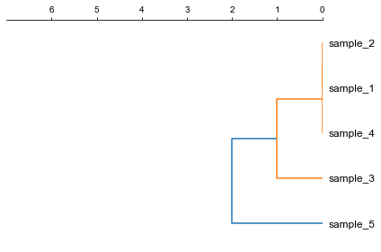
### 1. Plot a rectangular dendrogram
```python
fig, ax= plt.subplots(1,1)
lableorder, ax = cvmplot.rectree(link_matrix, scale_max=7, labels=samples, ax=ax)
fig.tight_layout()
fig.savefig('screenshots/dendrogram.png')
```
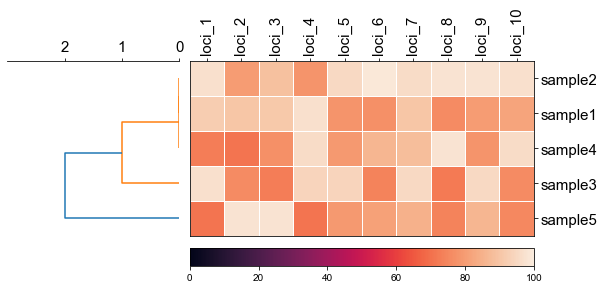
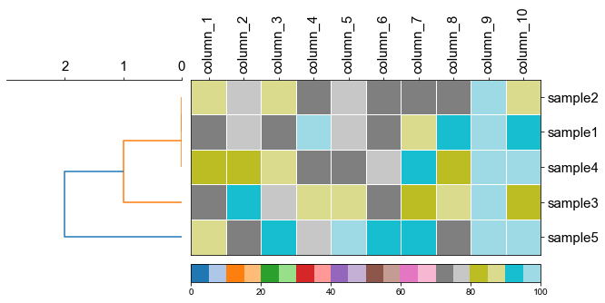
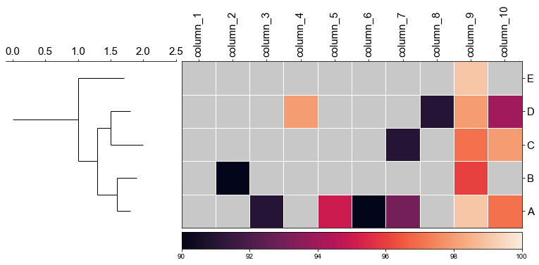
### 2. Plot rectangular dendrogram with heatmap
```python
#create dataframe
mat = np.random.randint(70, 100, (5, 10))
loci = np.char.replace(np.array(np.arange(1, 11), dtype='str'), '', 'loci_', count=1)
sample = np.char.replace(np.array(np.arange(1, 6), dtype='str'), '', 'sample', count=1)
df_heatmap = pd.DataFrame(mat, index=sample, columns=loci)
```
```python
#create linkage matrix
diff_matrix = [[0, 0, 1, 0, 1],
[0, 0, 1, 0, 1],
[1, 1, 0, 1, 2],
[0, 0, 1, 0, 1],
[1, 1, 2, 1, 0]]
linkage_matrix = linkage(squareform(diff_matrix),'complete')
```
```python
fig, (ax1, ax2) = plt.subplots(1,2,figsize=(8,3), gridspec_kw={'width_ratios': [1, 2]})
fig.tight_layout(w_pad=-2)
row_order, ax1 = cvmplot.rectree(linkage_matrix,labels=sample, no_labels=True, scale_max=3, ax=ax1)
cvmplot.heatmap(df_heatmap, order=row_order, ax=ax2, cbar=True, yticklabel=False)
ax1.set_xticklabels(ax1.get_xticklabels(), fontsize=15)
ax2.set_xticklabels(ax2.get_xticklabels(), rotation=90, fontsize=15)
ax2.set_yticklabels(ax2.get_yticklabels(), fontsize=15)
ax2.xaxis.tick_top()
# fig.tight_layout()
fig.savefig('screenshots/dendrogram_with_heatmap.png', bbox_inches='tight')
```
[ 5 15 25 35 45]
['sample5', 'sample3', 'sample4', 'sample1', 'sample2']
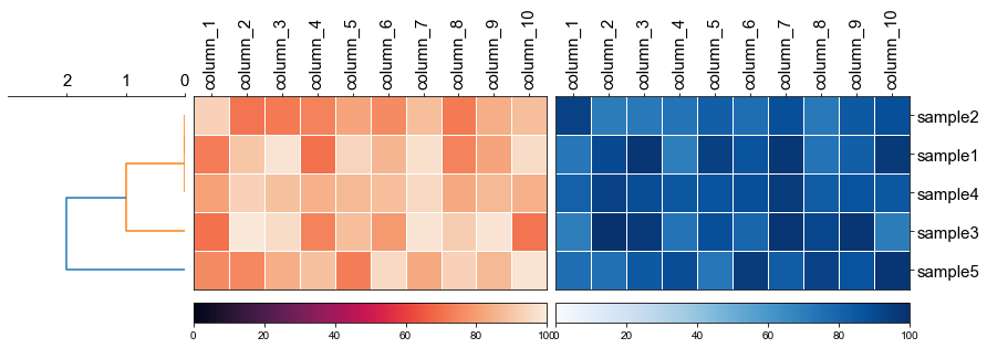
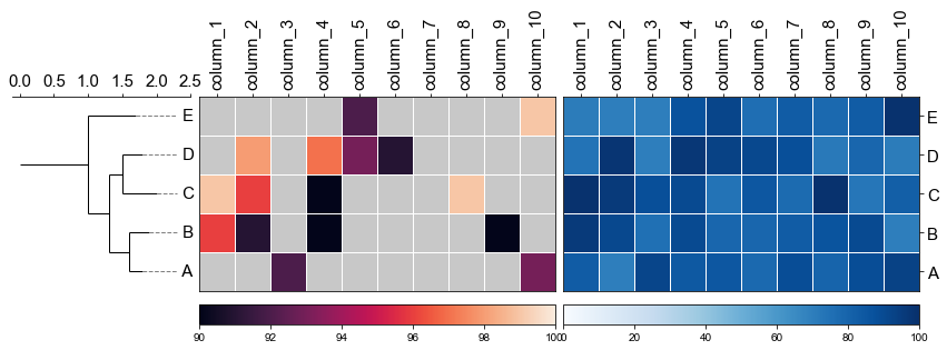
```python
fig, (ax1, ax2, ax3) = plt.subplots(1,3,figsize=(12,3), gridspec_kw={'width_ratios': [1, 2, 2]})
fig.tight_layout(w_pad=-2)
row_order, ax1 = cvmplot.rectree(linkage_matrix,labels=sample, no_labels=True, scale_max=3, ax=ax1)
# remove the yticklabels in ax2
ax2 = cvmplot.heatmap(df_heatmap, order=row_order, ax=ax2, cbar=True, yticklabel=False)
# add ax3 heatmap
ax3 = cvmplot.heatmap(df_heatmap, order=row_order, ax=ax3, cmap='Blues', cbar=True, yticklabel=True)
#set ticklabels property of x or y from ax1, ax2, ax3
ax1.set_xticklabels(ax1.get_xticklabels(), fontsize=15)
ax2.set_xticklabels(ax2.get_xticklabels(), rotation=90, fontsize=15)
ax2.xaxis.tick_top()
ax3.set_xticklabels(ax3.get_xticklabels(), rotation=90, fontsize=15)
ax3.set_yticklabels(ax3.get_yticklabels(), fontsize=15)
ax3.xaxis.tick_top()
# fig.tight_layout()
fig.savefig('screenshots/multiple_heatmap.png', bbox_inches='tight')
```
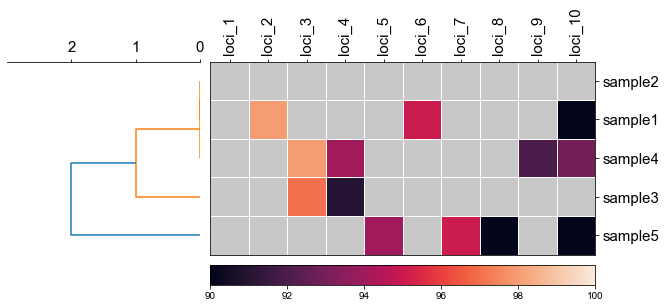
#### 2.1 set minimum value of heatmap
```python
fig, (ax1, ax2) = plt.subplots(1,2,figsize=(8,3), gridspec_kw={'width_ratios': [1, 2]})
fig.tight_layout(w_pad=-2)
order, ax1 = cvmplot.rectree(linkage_matrix,labels=sample, no_labels=True, scale_max=3, ax=ax1)
cvmplot.heatmap(df_heatmap, order=order, ax=ax2, cbar=True, vmin=90)
ax1.set_xticklabels(ax1.get_xticklabels(), fontsize=15)
ax2.set_xticklabels(ax2.get_xticklabels(), rotation=90, fontsize=15)
ax2.set_yticklabels(ax2.get_yticklabels(), fontsize=15)
ax2.xaxis.tick_top()
fig.savefig('screenshots/dendrogram_heatmap_minimumvalue.pdf', bbox_inches='tight')
```
[ 5 15 25 35 45]
['sample5', 'sample3', 'sample4', 'sample1', 'sample2']
#### 2.2 using cmap to change color
```python
fig, (ax1, ax2) = plt.subplots(1,2,figsize=(8,3), gridspec_kw={'width_ratios': [1, 2]})
fig.tight_layout(w_pad=-2)
order, ax1 = cvmplot.rectree(linkage_matrix,labels=sample, no_labels=True, scale_max=3, ax=ax1)
cvmplot.heatmap(df_heatmap, order=order, ax=ax2, cmap='tab20', cbar=True)
ax1.set_xticklabels(ax1.get_xticklabels(), fontsize=15)
ax2.set_xticklabels(ax2.get_xticklabels(), rotation=90, fontsize=15)
ax2.set_yticklabels(ax2.get_yticklabels(), fontsize=15)
ax2.xaxis.tick_top()
fig.savefig('screenshots/dendrogram_heatmap_cmap.pdf', bbox_inches='tight')
```
[ 5 15 25 35 45]
['sample5', 'sample3', 'sample4', 'sample1', 'sample2']
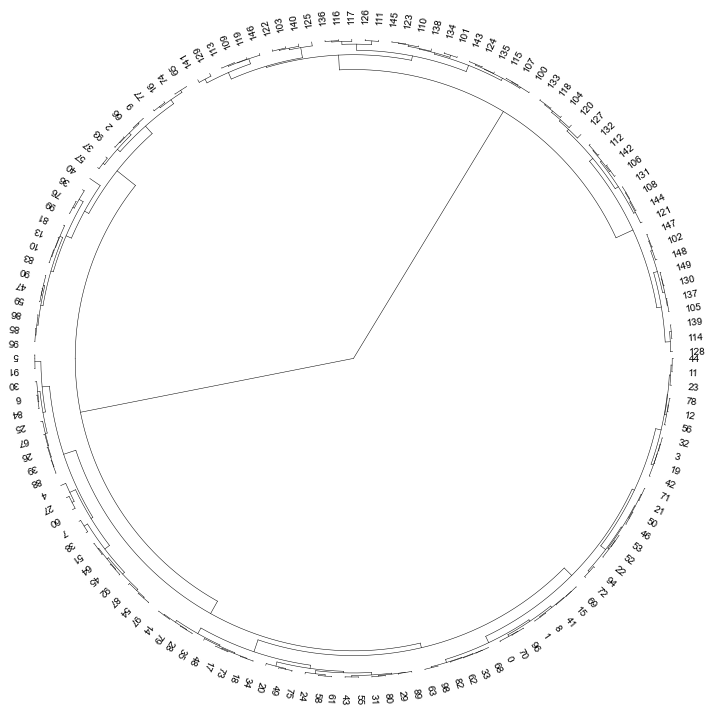
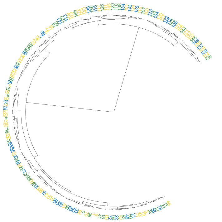
### 3. Plot a circular dendrogram
```python
# generate two clusters: a with 100 points, b with 50:
np.random.seed(4711) # for repeatability of this tutorial
a = np.random.multivariate_normal([10, 0], [[3, 1], [1, 4]], size=[100,])
b = np.random.multivariate_normal([0, 20], [[3, 1], [1, 4]], size=[50,])
X = np.concatenate((a, b),)
```
```python
Z = linkage(X, 'ward')
```
```python
Z2 = dendrogram(Z, no_plot=True)
```
```python
# set open angle
fig, ax= plt.subplots(1,1,figsize=(10,10))
cvmplot.circulartree(Z2,addlabels=True, fontsize=10, ax=ax)
fig.tight_layout()
fig.savefig('screenshots/circular_dendrogram.png', bbox_inches='tight')
```
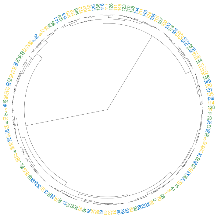
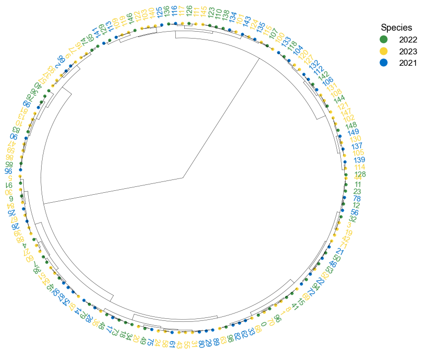
#### 3.1 color label
```python
colors = [{'#0070c7':'2021'}, {'#3a9245':'2022'}, {'#f8d438':'2023'}]
result = np.random.choice(colors, size=150)
label_colors_map = dict(zip(Z2['ivl'], result))
point_colors_map = dict(zip(Z2['ivl'], result))
```
```python
fig, ax= plt.subplots(1,1,figsize=(10,10))
cvmplot.circulartree(Z2, addlabels=True, branch_color=False, label_colors= label_colors_map, fontsize=15)
fig.tight_layout()
fig.savefig('screenshots/circular_dendrogram_color_label.png')
```
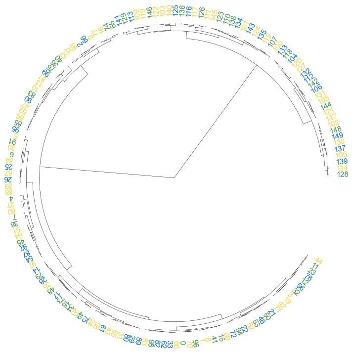
#### 3.2 set open angle
```python
fig, ax= plt.subplots(1,1,figsize=(10,10))
cvmplot.circulartree(Z2, addlabels=True, branch_color=False, label_colors= label_colors_map, fontsize=15, open_angle=30)
fig.tight_layout()
fig.savefig('screenshots/circular_dendrogram_openangle.png')
```
#### 3.3 set start angle
```python
fig, ax= plt.subplots(1,1,figsize=(10,10))
cvmplot.circulartree(Z2, addlabels=True, branch_color=False, label_colors= label_colors_map, fontsize=15, open_angle=90,
start_angle=30
)
fig.tight_layout()
fig.savefig('screenshots/circular_dendrogram_startangle.png')
```
#### 3.4 add point
```python
fig, ax= plt.subplots(1,1,figsize=(12,10))
cvmplot.circulartree(Z2, addlabels=True, branch_color=False, label_colors= label_colors_map, fontsize=15, addpoints=True,
point_colors = point_colors_map, point_legend_title='Species', pointsize=25)
fig.tight_layout()
fig.savefig('screenshots/circular_dendrogram_tippoints.png')
```
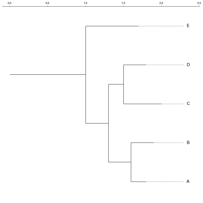
### 4. Plot phylogenetic tree
```python
tree = "(((A:0.2, B:0.3):0.3,(C:0.5, D:0.3):0.2):0.3, E:0.7):1.0;"
tree = Phylo.read(StringIO(tree), 'newick')
```
```python
fig, ax= plt.subplots(1,1, figsize=(10, 10))
ax, lable_order = cvmplot.phylotree(tree=tree, color='k', lw=1, ax=ax, show_label=True, align_label=True, labelsize=15)
fig.tight_layout()
fig.savefig('screenshots/phylogenetic tree.png')
```
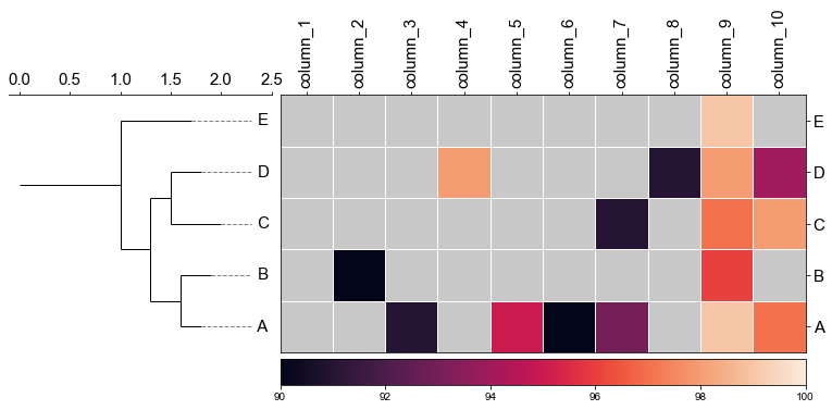
#### 4.1 Plot tree with heatmap
```python
#create dataframe
mat = np.random.randint(70, 100, (5, 10))
col = np.char.replace(np.array(np.arange(1, 11), dtype='str'), '', 'column_', count=1)
strains = ['A', 'B', 'C', 'D', 'E']
df_heatmap = pd.DataFrame(mat, index=strains, columns=col)
```
```python
df_heatmap
```
<div>
<table border="1" class="dataframe">
<thead>
<tr style="text-align: right;">
<th></th>
<th>column_1</th>
<th>column_2</th>
<th>column_3</th>
<th>column_4</th>
<th>column_5</th>
<th>column_6</th>
<th>column_7</th>
<th>column_8</th>
<th>column_9</th>
<th>column_10</th>
</tr>
</thead>
<tbody>
<tr>
<th>A</th>
<td>89</td>
<td>73</td>
<td>91</td>
<td>75</td>
<td>95</td>
<td>90</td>
<td>93</td>
<td>74</td>
<td>99</td>
<td>97</td>
</tr>
<tr>
<th>B</th>
<td>73</td>
<td>90</td>
<td>75</td>
<td>89</td>
<td>85</td>
<td>72</td>
<td>82</td>
<td>85</td>
<td>96</td>
<td>82</td>
</tr>
<tr>
<th>C</th>
<td>84</td>
<td>82</td>
<td>86</td>
<td>74</td>
<td>72</td>
<td>75</td>
<td>91</td>
<td>83</td>
<td>97</td>
<td>98</td>
</tr>
<tr>
<th>D</th>
<td>72</td>
<td>77</td>
<td>72</td>
<td>98</td>
<td>79</td>
<td>73</td>
<td>87</td>
<td>91</td>
<td>98</td>
<td>94</td>
</tr>
<tr>
<th>E</th>
<td>88</td>
<td>75</td>
<td>88</td>
<td>73</td>
<td>77</td>
<td>72</td>
<td>74</td>
<td>73</td>
<td>99</td>
<td>86</td>
</tr>
</tbody>
</table>
</div>
```python
fig,(ax1, ax2)= plt.subplots(1,2, figsize=(8, 3), gridspec_kw={'width_ratios':[1, 2]})
fig.tight_layout(w_pad=-2)
ax1, order = cvmplot.phylotree(tree=tree, color='k', lw=1, ax=ax1, show_label=True, align_label=True, labelsize=15)
cvmplot.heatmap(df_heatmap, order=order, ax=ax2, cbar=True, vmin=90)
ax1.set_xticklabels(ax1.get_xticklabels(), fontsize=15)
ax2.set_xticklabels(ax2.get_xticklabels(), rotation=90, fontsize=15)
ax2.set_yticklabels(ax2.get_yticklabels(), fontsize=15)
ax2.xaxis.tick_top()
fig.savefig('screenshots/phylotree_with_heatmap.pdf')
```
#### 4.2 remove labels at the tip of the tree
```python
fig,(ax1, ax2)= plt.subplots(1,2, figsize=(8, 3), gridspec_kw={'width_ratios':[1, 2]})
fig.tight_layout(w_pad=-2)
ax1, order = cvmplot.phylotree(tree=tree, color='k', lw=1, ax=ax1, show_label=False)
cvmplot.heatmap(df_heatmap, order=order, ax=ax2, cbar=True, vmin=90)
ax1.set_xticklabels(ax1.get_xticklabels(), fontsize=15)
ax2.set_xticklabels(ax2.get_xticklabels(), rotation=90, fontsize=15)
ax2.set_yticklabels(ax2.get_yticklabels(), fontsize=15)
ax2.xaxis.tick_top()
fig.savefig('screenshots/phylotree_with_heatmap-remove_tiplable.pdf', bbox_inches='tight')
```
#### 4.3 Plot multiple heatmap with phylotree
```
fig,(ax1, ax2, ax3)= plt.subplots(1,3, figsize=(12, 3), gridspec_kw={'width_ratios':[1, 2, 2]})
fig.tight_layout(w_pad=-2)
ax1, order = cvmplot.phylotree(tree=tree, color='k', lw=1, ax=ax1, show_label=True, align_label=True, labelsize=15)
ax2 = cvmplot.heatmap(df_heatmap, order=order, ax=ax2, cbar=True, vmin=90, yticklabel=False)
# add ax3 heatmap
ax3 = cvmplot.heatmap(df_heatmap, order=order, ax=ax3, cmap='Blues', cbar=True, yticklabel=True)
#set ticklabels property of x or y from ax1, ax2, ax3
ax1.set_xticklabels(ax1.get_xticklabels(), fontsize=15)
ax2.set_xticklabels(ax2.get_xticklabels(), rotation=90, fontsize=15)
ax2.xaxis.tick_top()
ax3.set_xticklabels(ax3.get_xticklabels(), rotation=90, fontsize=15)
ax3.set_yticklabels(ax3.get_yticklabels(), fontsize=15)
ax3.xaxis.tick_top()
# fig.tight_layout()
fig.savefig('screenshots/phylotree_multiple_heatmap.png', bbox_inches='tight')
```
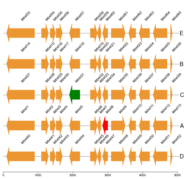
### 5. Gene environment plot
First, you shoud prepare a dataframe from the gff file, The columns should include the feature start, end, strand, label(gene name or whatever you want show next to the arrow) and the arrow color.
|TRACK|START|END|STRAND|LABEL|COLOR|
|---|------|------|----|---------|---------|
| A | 100 | 900 | -1 | label1 | #ec9631 |
| A | 1100 | 1300 | 1 | label2 | #ec9631 |
| A | 1350 | 1500 | 1 | label3 | #ec9631 |
| A | 1520 | 1700 | 1 | label4 | #ec9631 |
| A | 1900 | 2200 | -1 | label5 | #ec9631 |
| A | 2500 | 2700 | 1 | label6 | #ec9631 |
| A | 2700 | 2800 | -1 | label7 | #ec9631 |
| A | 2850 | 3000 | -1 | label8 | red |
| A | 3100 | 3500 | 1 | label9 | #ec9631 |
| A | 3600 | 3800 | -1 | label10 | #ec9631 |
| A | 3900 | 4200 | -1 | label11 | #ec9631 |
| A | 4300 | 4700 | -1 | label12 | #ec9631 |
| A | 4800 | 4850 | 1 | label13 | #ec9631 |
| B | 100 | 900 | -1 | label14 | #ec9631 |
| B | 1100 | 1300 | 1 | label15 | #ec9631 |
| B | 1350 | 1500 | 1 | label16 | #ec9631 |
| B | 1520 | 1700 | 1 | label17 | #ec9631 |
| B | 1900 | 2200 | -1 | label18 | #ec9631 |
| B | 2500 | 2700 | 1 | label19 | #ec9631 |
| B | 2700 | 2800 | -1 | label20 | #ec9631 |
| B | 2850 | 3000 | -1 | label21 | #ec9631 |
| B | 3100 | 3500 | 1 | label22 | #ec9631 |
| B | 3600 | 3800 | -1 | label23 | #ec9631 |
| B | 3900 | 4200 | -1 | label24 | #ec9631 |
| B | 4300 | 4700 | -1 | label25 | #ec9631 |
| B | 4800 | 4850 | 1 | label26 | #ec9631 |
| C | 100 | 900 | -1 | label27 | #ec9631 |
| C | 1100 | 1300 | 1 | label28 | #ec9631 |
| C | 1350 | 1500 | 1 | label29 | #ec9631 |
| C | 1520 | 1700 | 1 | label30 | #ec9631 |
| C | 1900 | 2200 | -1 | label31 | green |
| C | 2500 | 2700 | 1 | label32 | #ec9631 |
| C | 2700 | 2800 | -1 | label33 | #ec9631 |
| C | 2850 | 3000 | -1 | label34 | #ec9631 |
| C | 3100 | 3500 | 1 | label35 | #ec9631 |
| C | 3600 | 3800 | -1 | label36 | #ec9631 |
| C | 3900 | 4200 | -1 | label37 | #ec9631 |
| C | 4300 | 4700 | -1 | label38 | #ec9631 |
| C | 4800 | 4850 | 1 | label39 | #ec9631 |
| D | 100 | 900 | -1 | label40 | #ec9631 |
| D | 1100 | 1300 | 1 | label41 | #ec9631 |
| D | 1350 | 1500 | 1 | label42 | #ec9631 |
| D | 1520 | 1700 | 1 | label43 | #ec9631 |
| D | 1900 | 2200 | -1 | label44 | #ec9631 |
| D | 2500 | 2700 | 1 | label45 | #ec9631 |
| D | 2700 | 2800 | -1 | label46 | #ec9631 |
| D | 2850 | 3000 | -1 | label47 | #ec9631 |
| D | 3100 | 3500 | 1 | label48 | #ec9631 |
| D | 3600 | 3800 | -1 | label49 | #ec9631 |
| D | 3900 | 4200 | -1 | label50 | #ec9631 |
| D | 4300 | 4700 | -1 | label51 | #ec9631 |
| D | 4800 | 4850 | 1 | label52 | #ec9631 |
| E | 100 | 900 | -1 | label53 | #ec9631 |
| E | 1100 | 1300 | 1 | label54 | #ec9631 |
| E | 1350 | 1500 | 1 | label55 | #ec9631 |
| E | 1520 | 1700 | 1 | label56 | #ec9631 |
| E | 1900 | 2200 | -1 | label57 | #ec9631 |
| E | 2500 | 2700 | 1 | label58 | #ec9631 |
| E | 2700 | 2800 | -1 | label59 | #ec9631 |
| E | 2850 | 3000 | -1 | label60 | #ec9631 |
| E | 3100 | 3500 | 1 | label61 | #ec9631 |
| E | 3600 | 3800 | -1 | label62 | #ec9631 |
| E | 3900 | 4200 | -1 | label63 | #ec9631 |
| E | 4300 | 4700 | -1 | label64 | #ec9631 |
| E | 4800 | 4850 | 1 | label65 | #ec9631 |
### 5. Plot genes
```
# Create arrow dictionary
arrow_dict = {k: g.to_dict(orient='records') for k, g in df.set_index('TRACK').groupby(level=0)}
# Define the display order of your tracks
order = ['D', 'A', 'C', 'B', 'E']
```
#### 5.1 Plot gene arrows and label on top track
```
fig, ax = plt.subplots(1,1, figsize=(10,10))
ax = cvmplot.plotgenes(dc=arrow_dict, order=order, ax=ax, max_track_size=5000, addlabels=True, label_track='top')
fig.savefig('screenshots/gene_arrow_top.png', bbox_inches='tight')
```
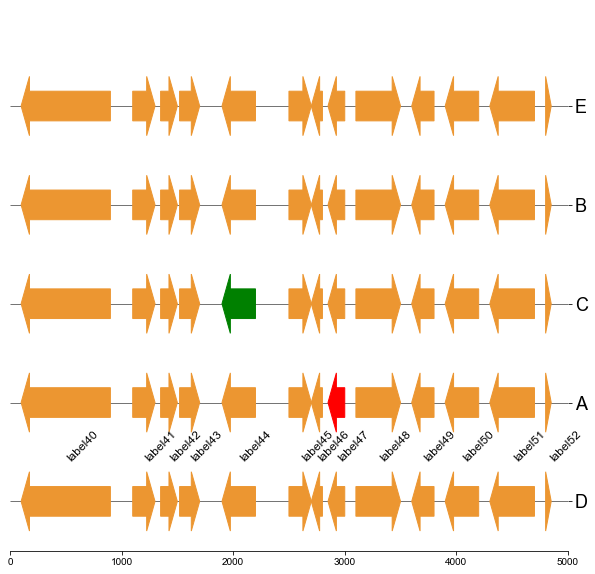
#### 5.2 Plot gene arrows and label on bottom track
```
fig, ax = plt.subplots(1,1, figsize=(10,10))
ax = cvmplot.plotgenes(dc=arrow_dict, order=order, ax=ax, max_track_size=5000, addlabels=True, label_track='bottom')
fig.savefig('screenshots/gene_arrow_bottom.png', bbox_inches='tight')
```
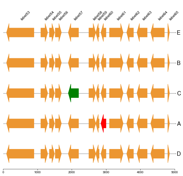
#### 5.3 Plot gene arrows and label on all tracks
```
fig, ax = plt.subplots(1,1, figsize=(10,10))
ax = cvmplot.plotgenes(dc=arrow_dict, order=order, ax=ax, max_track_size=5000, addlabels=True, label_track='all')
fig.savefig('screenshots/gene_arrow_all.png', bbox_inches='tight')
```
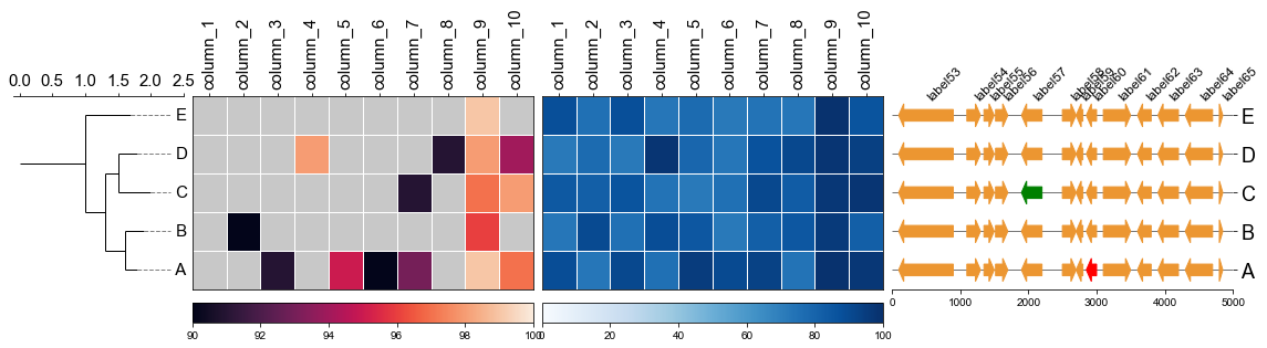
#### 5.4 Plot gene arrows with phylotree and heatmap
Put together!
```
# Put together
fig,(ax1, ax2, ax3, ax4)= plt.subplots(1,4, figsize=(16, 3), gridspec_kw={'width_ratios':[1, 2, 2, 2]})
fig.tight_layout(w_pad=-2)
ax1, order = cvmplot.phylotree(tree=tree, color='k', lw=1, ax=ax1, show_label=True, align_label=True, labelsize=15)
ax2 = cvmplot.heatmap(df_heatmap, order=order, ax=ax2, cbar=True, vmin=90, yticklabel=False)
# add ax3 heatmap
ax3 = cvmplot.heatmap(df_heatmap, order=order, ax=ax3, cmap='Blues', cbar=True, yticklabel=False)
ax4 = cvmplot.plotgenes(dc=arrow_dict, order=order, ax=ax4, max_track_size=5000, addlabels=True, label_track='top', ylim=(-3, 3))
#set ticklabels property of x or y from ax1, ax2, ax3
ax1.set_xticklabels(ax1.get_xticklabels(), fontsize=15)
ax2.set_xticklabels(ax2.get_xticklabels(), rotation=90, fontsize=15)
ax2.xaxis.tick_top()
ax3.set_xticklabels(ax3.get_xticklabels(), rotation=90, fontsize=15)
ax3.set_yticklabels(ax3.get_yticklabels(), fontsize=15)
ax3.xaxis.tick_top()
# fig.tight_layout()
fig.savefig('screenshots/phylotree_heatmap_withgenes.png', bbox_inches='tight')
```
Raw data
{
"_id": null,
"home_page": "https://github.com/hbucqp/cvmcore",
"name": "cvmcore",
"maintainer": "",
"docs_url": null,
"requires_python": "",
"maintainer_email": "",
"keywords": "pip,mlst,cgmlst,plot",
"author": "Qingpo Cui",
"author_email": "cqp@cau.edu.cn",
"download_url": "https://files.pythonhosted.org/packages/d9/ce/aa44f57f09dd55db71dd0ed90fb8ec0418cd2637f97760d89ab8c17440f9/cvmcore-0.1.2.tar.gz",
"platform": "any",
"description": "# cvmcore\n\n\n\n\n## Introduction\nThe core function of data analysis for plot or data process used by SZQ lab from China Agricultural University\n\n\n## Example usage\n\n\n```python\nfrom Bio import Phylo\nimport matplotlib as mpl\nimport matplotlib.pyplot as plt\nfrom io import StringIO\nimport matplotlib.collections as mpcollections\nfrom copy import copy\n\nimport pandas as pd\nimport numpy as np\nimport seaborn as sn\n\nfrom cvmcore.cvmcore import cvmplot\n\nfrom scipy.cluster.hierarchy import linkage, dendrogram, complete, to_tree\nfrom scipy.spatial.distance import squareform\n```\n\n\n```python\nmlst = [[np.nan, 19., 12., 9., 5., 9., 2.],\n [np.nan, 19., 12., 9., 5., 9., 2.],\n [10., 17., 12., 9., np.nan, 9., 2.],\n [10., 19., 12., np.nan, 5., 9., 2.],\n [np.nan, 19., 13., 9., 5., 9., 2.]]\ngenes = np.char.replace(np.array(np.arange(1, 8), dtype='str'), '', 'gene_', count=1)\nsamples = np.char.replace(np.array(np.arange(1, 6), dtype='str'), '', 'sample_', count=1)\ndf_mlst = pd.DataFrame(mlst, index=samples, columns=genes)\ndiff_matrix = cvmplot.get_diff_df(df_mlst)\n```\n\n\n```python\ndiff_matrix\n```\n\n\n\n\n<div>\n<table border=\"1\" class=\"dataframe\">\n <thead>\n <tr style=\"text-align: right;\">\n <th></th>\n <th>sample_1</th>\n <th>sample_2</th>\n <th>sample_3</th>\n <th>sample_4</th>\n <th>sample_5</th>\n </tr>\n </thead>\n <tbody>\n <tr>\n <th>sample_1</th>\n <td>0</td>\n <td>0</td>\n <td>1</td>\n <td>0</td>\n <td>1</td>\n </tr>\n <tr>\n <th>sample_2</th>\n <td>0</td>\n <td>0</td>\n <td>1</td>\n <td>0</td>\n <td>1</td>\n </tr>\n <tr>\n <th>sample_3</th>\n <td>1</td>\n <td>1</td>\n <td>0</td>\n <td>1</td>\n <td>2</td>\n </tr>\n <tr>\n <th>sample_4</th>\n <td>0</td>\n <td>0</td>\n <td>1</td>\n <td>0</td>\n <td>1</td>\n </tr>\n <tr>\n <th>sample_5</th>\n <td>1</td>\n <td>1</td>\n <td>2</td>\n <td>1</td>\n <td>0</td>\n </tr>\n </tbody>\n</table>\n</div>\n\n\n\n\n```python\nlink_matrix =linkage(squareform(diff_matrix), method='complete')\n```\n\n\n```python\nlink_matrix\n```\n\n\n\n\n array([[0., 1., 0., 2.],\n [3., 5., 0., 3.],\n [2., 6., 1., 4.],\n [4., 7., 2., 5.]])\n\n\n\n### 1. Plot a rectangular dendrogram\n\n\n```python\nfig, ax= plt.subplots(1,1)\nlableorder, ax = cvmplot.rectree(link_matrix, scale_max=7, labels=samples, ax=ax)\nfig.tight_layout()\nfig.savefig('screenshots/dendrogram.png')\n```\n\n\n\n\n\n### 2. Plot rectangular dendrogram with heatmap\n\n\n```python\n#create dataframe\nmat = np.random.randint(70, 100, (5, 10))\nloci = np.char.replace(np.array(np.arange(1, 11), dtype='str'), '', 'loci_', count=1)\nsample = np.char.replace(np.array(np.arange(1, 6), dtype='str'), '', 'sample', count=1)\ndf_heatmap = pd.DataFrame(mat, index=sample, columns=loci)\n```\n\n\n```python\n#create linkage matrix\ndiff_matrix = [[0, 0, 1, 0, 1],\n [0, 0, 1, 0, 1],\n [1, 1, 0, 1, 2],\n [0, 0, 1, 0, 1],\n [1, 1, 2, 1, 0]]\n\nlinkage_matrix = linkage(squareform(diff_matrix),'complete')\n```\n\n\n```python\nfig, (ax1, ax2) = plt.subplots(1,2,figsize=(8,3), gridspec_kw={'width_ratios': [1, 2]})\n\nfig.tight_layout(w_pad=-2)\n\nrow_order, ax1 = cvmplot.rectree(linkage_matrix,labels=sample, no_labels=True, scale_max=3, ax=ax1)\ncvmplot.heatmap(df_heatmap, order=row_order, ax=ax2, cbar=True, yticklabel=False)\n\nax1.set_xticklabels(ax1.get_xticklabels(), fontsize=15)\n\nax2.set_xticklabels(ax2.get_xticklabels(), rotation=90, fontsize=15)\nax2.set_yticklabels(ax2.get_yticklabels(), fontsize=15)\nax2.xaxis.tick_top()\n\n# fig.tight_layout()\nfig.savefig('screenshots/dendrogram_with_heatmap.png', bbox_inches='tight')\n```\n\n [ 5 15 25 35 45]\n ['sample5', 'sample3', 'sample4', 'sample1', 'sample2']\n\n\n\n\n\n```python\nfig, (ax1, ax2, ax3) = plt.subplots(1,3,figsize=(12,3), gridspec_kw={'width_ratios': [1, 2, 2]})\n\nfig.tight_layout(w_pad=-2)\n\nrow_order, ax1 = cvmplot.rectree(linkage_matrix,labels=sample, no_labels=True, scale_max=3, ax=ax1)\n\n# remove the yticklabels in ax2\nax2 = cvmplot.heatmap(df_heatmap, order=row_order, ax=ax2, cbar=True, yticklabel=False)\n# add ax3 heatmap\nax3 = cvmplot.heatmap(df_heatmap, order=row_order, ax=ax3, cmap='Blues', cbar=True, yticklabel=True)\n\n#set ticklabels property of x or y from ax1, ax2, ax3\nax1.set_xticklabels(ax1.get_xticklabels(), fontsize=15)\n\nax2.set_xticklabels(ax2.get_xticklabels(), rotation=90, fontsize=15)\nax2.xaxis.tick_top()\n\nax3.set_xticklabels(ax3.get_xticklabels(), rotation=90, fontsize=15)\nax3.set_yticklabels(ax3.get_yticklabels(), fontsize=15)\nax3.xaxis.tick_top()\n\n\n# fig.tight_layout()\nfig.savefig('screenshots/multiple_heatmap.png', bbox_inches='tight')\n```\n\n\n#### 2.1 set minimum value of heatmap\n\n\n```python\nfig, (ax1, ax2) = plt.subplots(1,2,figsize=(8,3), gridspec_kw={'width_ratios': [1, 2]})\nfig.tight_layout(w_pad=-2)\n\norder, ax1 = cvmplot.rectree(linkage_matrix,labels=sample, no_labels=True, scale_max=3, ax=ax1)\ncvmplot.heatmap(df_heatmap, order=order, ax=ax2, cbar=True, vmin=90)\n\nax1.set_xticklabels(ax1.get_xticklabels(), fontsize=15)\n\nax2.set_xticklabels(ax2.get_xticklabels(), rotation=90, fontsize=15)\nax2.set_yticklabels(ax2.get_yticklabels(), fontsize=15)\nax2.xaxis.tick_top()\n\nfig.savefig('screenshots/dendrogram_heatmap_minimumvalue.pdf', bbox_inches='tight')\n```\n\n [ 5 15 25 35 45]\n ['sample5', 'sample3', 'sample4', 'sample1', 'sample2']\n\n\n\n\n\n\n#### 2.2 using cmap to change color\n\n\n```python\nfig, (ax1, ax2) = plt.subplots(1,2,figsize=(8,3), gridspec_kw={'width_ratios': [1, 2]})\nfig.tight_layout(w_pad=-2)\n\norder, ax1 = cvmplot.rectree(linkage_matrix,labels=sample, no_labels=True, scale_max=3, ax=ax1)\ncvmplot.heatmap(df_heatmap, order=order, ax=ax2, cmap='tab20', cbar=True)\n\nax1.set_xticklabels(ax1.get_xticklabels(), fontsize=15)\n\nax2.set_xticklabels(ax2.get_xticklabels(), rotation=90, fontsize=15)\nax2.set_yticklabels(ax2.get_yticklabels(), fontsize=15)\nax2.xaxis.tick_top()\nfig.savefig('screenshots/dendrogram_heatmap_cmap.pdf', bbox_inches='tight')\n```\n\n [ 5 15 25 35 45]\n ['sample5', 'sample3', 'sample4', 'sample1', 'sample2']\n\n\n\n\n\n\n### 3. Plot a circular dendrogram\n\n\n```python\n# generate two clusters: a with 100 points, b with 50:\nnp.random.seed(4711) # for repeatability of this tutorial\na = np.random.multivariate_normal([10, 0], [[3, 1], [1, 4]], size=[100,])\nb = np.random.multivariate_normal([0, 20], [[3, 1], [1, 4]], size=[50,])\nX = np.concatenate((a, b),)\n```\n\n\n```python\nZ = linkage(X, 'ward')\n```\n\n\n```python\nZ2 = dendrogram(Z, no_plot=True)\n```\n\n\n```python\n# set open angle\nfig, ax= plt.subplots(1,1,figsize=(10,10))\n\ncvmplot.circulartree(Z2,addlabels=True, fontsize=10, ax=ax)\nfig.tight_layout()\nfig.savefig('screenshots/circular_dendrogram.png', bbox_inches='tight')\n```\n\n\n\n\n\n#### 3.1 color label\n\n\n```python\ncolors = [{'#0070c7':'2021'}, {'#3a9245':'2022'}, {'#f8d438':'2023'}]\nresult = np.random.choice(colors, size=150)\nlabel_colors_map = dict(zip(Z2['ivl'], result))\npoint_colors_map = dict(zip(Z2['ivl'], result))\n```\n\n\n```python\nfig, ax= plt.subplots(1,1,figsize=(10,10))\ncvmplot.circulartree(Z2, addlabels=True, branch_color=False, label_colors= label_colors_map, fontsize=15)\nfig.tight_layout()\nfig.savefig('screenshots/circular_dendrogram_color_label.png')\n```\n\n\n\n\n\n#### 3.2 set open angle\n\n\n```python\nfig, ax= plt.subplots(1,1,figsize=(10,10))\ncvmplot.circulartree(Z2, addlabels=True, branch_color=False, label_colors= label_colors_map, fontsize=15, open_angle=30)\nfig.tight_layout()\nfig.savefig('screenshots/circular_dendrogram_openangle.png')\n```\n\n\n\n\n\n#### 3.3 set start angle\n\n\n```python\nfig, ax= plt.subplots(1,1,figsize=(10,10))\ncvmplot.circulartree(Z2, addlabels=True, branch_color=False, label_colors= label_colors_map, fontsize=15, open_angle=90,\n start_angle=30\n )\nfig.tight_layout()\nfig.savefig('screenshots/circular_dendrogram_startangle.png')\n```\n\n\n\n\n\n#### 3.4 add point \n\n\n```python\nfig, ax= plt.subplots(1,1,figsize=(12,10))\ncvmplot.circulartree(Z2, addlabels=True, branch_color=False, label_colors= label_colors_map, fontsize=15, addpoints=True,\n point_colors = point_colors_map, point_legend_title='Species', pointsize=25)\nfig.tight_layout()\nfig.savefig('screenshots/circular_dendrogram_tippoints.png')\n```\n\n\n\n\n\n\n### 4. Plot phylogenetic tree\n\n\n```python\ntree = \"(((A:0.2, B:0.3):0.3,(C:0.5, D:0.3):0.2):0.3, E:0.7):1.0;\"\ntree = Phylo.read(StringIO(tree), 'newick')\n```\n\n\n```python\nfig, ax= plt.subplots(1,1, figsize=(10, 10))\nax, lable_order = cvmplot.phylotree(tree=tree, color='k', lw=1, ax=ax, show_label=True, align_label=True, labelsize=15)\nfig.tight_layout()\nfig.savefig('screenshots/phylogenetic tree.png')\n```\n\n\n\n\n\n#### 4.1 Plot tree with heatmap\n\n\n```python\n#create dataframe\nmat = np.random.randint(70, 100, (5, 10))\ncol = np.char.replace(np.array(np.arange(1, 11), dtype='str'), '', 'column_', count=1)\nstrains = ['A', 'B', 'C', 'D', 'E']\ndf_heatmap = pd.DataFrame(mat, index=strains, columns=col)\n```\n\n\n```python\ndf_heatmap\n```\n\n\n\n\n<div>\n<table border=\"1\" class=\"dataframe\">\n <thead>\n <tr style=\"text-align: right;\">\n <th></th>\n <th>column_1</th>\n <th>column_2</th>\n <th>column_3</th>\n <th>column_4</th>\n <th>column_5</th>\n <th>column_6</th>\n <th>column_7</th>\n <th>column_8</th>\n <th>column_9</th>\n <th>column_10</th>\n </tr>\n </thead>\n <tbody>\n <tr>\n <th>A</th>\n <td>89</td>\n <td>73</td>\n <td>91</td>\n <td>75</td>\n <td>95</td>\n <td>90</td>\n <td>93</td>\n <td>74</td>\n <td>99</td>\n <td>97</td>\n </tr>\n <tr>\n <th>B</th>\n <td>73</td>\n <td>90</td>\n <td>75</td>\n <td>89</td>\n <td>85</td>\n <td>72</td>\n <td>82</td>\n <td>85</td>\n <td>96</td>\n <td>82</td>\n </tr>\n <tr>\n <th>C</th>\n <td>84</td>\n <td>82</td>\n <td>86</td>\n <td>74</td>\n <td>72</td>\n <td>75</td>\n <td>91</td>\n <td>83</td>\n <td>97</td>\n <td>98</td>\n </tr>\n <tr>\n <th>D</th>\n <td>72</td>\n <td>77</td>\n <td>72</td>\n <td>98</td>\n <td>79</td>\n <td>73</td>\n <td>87</td>\n <td>91</td>\n <td>98</td>\n <td>94</td>\n </tr>\n <tr>\n <th>E</th>\n <td>88</td>\n <td>75</td>\n <td>88</td>\n <td>73</td>\n <td>77</td>\n <td>72</td>\n <td>74</td>\n <td>73</td>\n <td>99</td>\n <td>86</td>\n </tr>\n </tbody>\n</table>\n</div>\n\n\n\n\n```python\nfig,(ax1, ax2)= plt.subplots(1,2, figsize=(8, 3), gridspec_kw={'width_ratios':[1, 2]})\nfig.tight_layout(w_pad=-2)\nax1, order = cvmplot.phylotree(tree=tree, color='k', lw=1, ax=ax1, show_label=True, align_label=True, labelsize=15)\ncvmplot.heatmap(df_heatmap, order=order, ax=ax2, cbar=True, vmin=90)\n\nax1.set_xticklabels(ax1.get_xticklabels(), fontsize=15)\n\nax2.set_xticklabels(ax2.get_xticklabels(), rotation=90, fontsize=15)\nax2.set_yticklabels(ax2.get_yticklabels(), fontsize=15)\nax2.xaxis.tick_top()\n\nfig.savefig('screenshots/phylotree_with_heatmap.pdf')\n```\n\n\n\n\n\n\n\n#### 4.2 remove labels at the tip of the tree\n\n\n```python\nfig,(ax1, ax2)= plt.subplots(1,2, figsize=(8, 3), gridspec_kw={'width_ratios':[1, 2]})\nfig.tight_layout(w_pad=-2)\nax1, order = cvmplot.phylotree(tree=tree, color='k', lw=1, ax=ax1, show_label=False)\ncvmplot.heatmap(df_heatmap, order=order, ax=ax2, cbar=True, vmin=90)\n\nax1.set_xticklabels(ax1.get_xticklabels(), fontsize=15)\n\nax2.set_xticklabels(ax2.get_xticklabels(), rotation=90, fontsize=15)\nax2.set_yticklabels(ax2.get_yticklabels(), fontsize=15)\nax2.xaxis.tick_top()\n\nfig.savefig('screenshots/phylotree_with_heatmap-remove_tiplable.pdf', bbox_inches='tight')\n```\n\n\n\n\n\n#### 4.3 Plot multiple heatmap with phylotree\n```\nfig,(ax1, ax2, ax3)= plt.subplots(1,3, figsize=(12, 3), gridspec_kw={'width_ratios':[1, 2, 2]})\nfig.tight_layout(w_pad=-2)\nax1, order = cvmplot.phylotree(tree=tree, color='k', lw=1, ax=ax1, show_label=True, align_label=True, labelsize=15)\nax2 = cvmplot.heatmap(df_heatmap, order=order, ax=ax2, cbar=True, vmin=90, yticklabel=False)\n# add ax3 heatmap\nax3 = cvmplot.heatmap(df_heatmap, order=order, ax=ax3, cmap='Blues', cbar=True, yticklabel=True)\n\n#set ticklabels property of x or y from ax1, ax2, ax3\nax1.set_xticklabels(ax1.get_xticklabels(), fontsize=15)\n\nax2.set_xticklabels(ax2.get_xticklabels(), rotation=90, fontsize=15)\nax2.xaxis.tick_top()\n\nax3.set_xticklabels(ax3.get_xticklabels(), rotation=90, fontsize=15)\nax3.set_yticklabels(ax3.get_yticklabels(), fontsize=15)\nax3.xaxis.tick_top()\n\n\n# fig.tight_layout()\nfig.savefig('screenshots/phylotree_multiple_heatmap.png', bbox_inches='tight')\n```\n\n\n\n\n### 5. Gene environment plot\n\nFirst, you shoud prepare a dataframe from the gff file, The columns should include the feature start, end, strand, label(gene name or whatever you want show next to the arrow) and the arrow color.\n|TRACK|START|END|STRAND|LABEL|COLOR|\n|---|------|------|----|---------|---------|\n| A | 100 | 900 | -1 | label1 | #ec9631 |\n| A | 1100 | 1300 | 1 | label2 | #ec9631 |\n| A | 1350 | 1500 | 1 | label3 | #ec9631 |\n| A | 1520 | 1700 | 1 | label4 | #ec9631 |\n| A | 1900 | 2200 | -1 | label5 | #ec9631 |\n| A | 2500 | 2700 | 1 | label6 | #ec9631 |\n| A | 2700 | 2800 | -1 | label7 | #ec9631 |\n| A | 2850 | 3000 | -1 | label8 | red |\n| A | 3100 | 3500 | 1 | label9 | #ec9631 |\n| A | 3600 | 3800 | -1 | label10 | #ec9631 |\n| A | 3900 | 4200 | -1 | label11 | #ec9631 |\n| A | 4300 | 4700 | -1 | label12 | #ec9631 |\n| A | 4800 | 4850 | 1 | label13 | #ec9631 |\n| B | 100 | 900 | -1 | label14 | #ec9631 |\n| B | 1100 | 1300 | 1 | label15 | #ec9631 |\n| B | 1350 | 1500 | 1 | label16 | #ec9631 |\n| B | 1520 | 1700 | 1 | label17 | #ec9631 |\n| B | 1900 | 2200 | -1 | label18 | #ec9631 |\n| B | 2500 | 2700 | 1 | label19 | #ec9631 |\n| B | 2700 | 2800 | -1 | label20 | #ec9631 |\n| B | 2850 | 3000 | -1 | label21 | #ec9631 |\n| B | 3100 | 3500 | 1 | label22 | #ec9631 |\n| B | 3600 | 3800 | -1 | label23 | #ec9631 |\n| B | 3900 | 4200 | -1 | label24 | #ec9631 |\n| B | 4300 | 4700 | -1 | label25 | #ec9631 |\n| B | 4800 | 4850 | 1 | label26 | #ec9631 |\n| C | 100 | 900 | -1 | label27 | #ec9631 |\n| C | 1100 | 1300 | 1 | label28 | #ec9631 |\n| C | 1350 | 1500 | 1 | label29 | #ec9631 |\n| C | 1520 | 1700 | 1 | label30 | #ec9631 |\n| C | 1900 | 2200 | -1 | label31 | green |\n| C | 2500 | 2700 | 1 | label32 | #ec9631 |\n| C | 2700 | 2800 | -1 | label33 | #ec9631 |\n| C | 2850 | 3000 | -1 | label34 | #ec9631 |\n| C | 3100 | 3500 | 1 | label35 | #ec9631 |\n| C | 3600 | 3800 | -1 | label36 | #ec9631 |\n| C | 3900 | 4200 | -1 | label37 | #ec9631 |\n| C | 4300 | 4700 | -1 | label38 | #ec9631 |\n| C | 4800 | 4850 | 1 | label39 | #ec9631 |\n| D | 100 | 900 | -1 | label40 | #ec9631 |\n| D | 1100 | 1300 | 1 | label41 | #ec9631 |\n| D | 1350 | 1500 | 1 | label42 | #ec9631 |\n| D | 1520 | 1700 | 1 | label43 | #ec9631 |\n| D | 1900 | 2200 | -1 | label44 | #ec9631 |\n| D | 2500 | 2700 | 1 | label45 | #ec9631 |\n| D | 2700 | 2800 | -1 | label46 | #ec9631 |\n| D | 2850 | 3000 | -1 | label47 | #ec9631 |\n| D | 3100 | 3500 | 1 | label48 | #ec9631 |\n| D | 3600 | 3800 | -1 | label49 | #ec9631 |\n| D | 3900 | 4200 | -1 | label50 | #ec9631 |\n| D | 4300 | 4700 | -1 | label51 | #ec9631 |\n| D | 4800 | 4850 | 1 | label52 | #ec9631 |\n| E | 100 | 900 | -1 | label53 | #ec9631 |\n| E | 1100 | 1300 | 1 | label54 | #ec9631 |\n| E | 1350 | 1500 | 1 | label55 | #ec9631 |\n| E | 1520 | 1700 | 1 | label56 | #ec9631 |\n| E | 1900 | 2200 | -1 | label57 | #ec9631 |\n| E | 2500 | 2700 | 1 | label58 | #ec9631 |\n| E | 2700 | 2800 | -1 | label59 | #ec9631 |\n| E | 2850 | 3000 | -1 | label60 | #ec9631 |\n| E | 3100 | 3500 | 1 | label61 | #ec9631 |\n| E | 3600 | 3800 | -1 | label62 | #ec9631 |\n| E | 3900 | 4200 | -1 | label63 | #ec9631 |\n| E | 4300 | 4700 | -1 | label64 | #ec9631 |\n| E | 4800 | 4850 | 1 | label65 | #ec9631 |\n\n\n### 5. Plot genes\n```\n# Create arrow dictionary\narrow_dict = {k: g.to_dict(orient='records') for k, g in df.set_index('TRACK').groupby(level=0)}\n\n# Define the display order of your tracks\norder = ['D', 'A', 'C', 'B', 'E']\n```\n#### 5.1 Plot gene arrows and label on top track\n```\nfig, ax = plt.subplots(1,1, figsize=(10,10))\nax = cvmplot.plotgenes(dc=arrow_dict, order=order, ax=ax, max_track_size=5000, addlabels=True, label_track='top')\nfig.savefig('screenshots/gene_arrow_top.png', bbox_inches='tight')\n```\n\n\n#### 5.2 Plot gene arrows and label on bottom track\n```\nfig, ax = plt.subplots(1,1, figsize=(10,10))\nax = cvmplot.plotgenes(dc=arrow_dict, order=order, ax=ax, max_track_size=5000, addlabels=True, label_track='bottom')\nfig.savefig('screenshots/gene_arrow_bottom.png', bbox_inches='tight')\n```\n\n\n\n#### 5.3 Plot gene arrows and label on all tracks\n\n```\nfig, ax = plt.subplots(1,1, figsize=(10,10))\nax = cvmplot.plotgenes(dc=arrow_dict, order=order, ax=ax, max_track_size=5000, addlabels=True, label_track='all')\nfig.savefig('screenshots/gene_arrow_all.png', bbox_inches='tight')\n\n```\n\n\n\n#### 5.4 Plot gene arrows with phylotree and heatmap\n\nPut together!\n```\n# Put together\nfig,(ax1, ax2, ax3, ax4)= plt.subplots(1,4, figsize=(16, 3), gridspec_kw={'width_ratios':[1, 2, 2, 2]})\nfig.tight_layout(w_pad=-2)\nax1, order = cvmplot.phylotree(tree=tree, color='k', lw=1, ax=ax1, show_label=True, align_label=True, labelsize=15)\nax2 = cvmplot.heatmap(df_heatmap, order=order, ax=ax2, cbar=True, vmin=90, yticklabel=False)\n# add ax3 heatmap\nax3 = cvmplot.heatmap(df_heatmap, order=order, ax=ax3, cmap='Blues', cbar=True, yticklabel=False)\n\nax4 = cvmplot.plotgenes(dc=arrow_dict, order=order, ax=ax4, max_track_size=5000, addlabels=True, label_track='top', ylim=(-3, 3))\n\n\n\n#set ticklabels property of x or y from ax1, ax2, ax3\nax1.set_xticklabels(ax1.get_xticklabels(), fontsize=15)\n\nax2.set_xticklabels(ax2.get_xticklabels(), rotation=90, fontsize=15)\nax2.xaxis.tick_top()\n\nax3.set_xticklabels(ax3.get_xticklabels(), rotation=90, fontsize=15)\nax3.set_yticklabels(ax3.get_yticklabels(), fontsize=15)\nax3.xaxis.tick_top()\n\n\n# fig.tight_layout()\nfig.savefig('screenshots/phylotree_heatmap_withgenes.png', bbox_inches='tight')\n```\n\n\n\n",
"bugtrack_url": null,
"license": "MIT Licence",
"summary": "SZQ lab data analysis core function",
"version": "0.1.2",
"project_urls": {
"Homepage": "https://github.com/hbucqp/cvmcore"
},
"split_keywords": [
"pip",
"mlst",
"cgmlst",
"plot"
],
"urls": [
{
"comment_text": "",
"digests": {
"blake2b_256": "e112b6f336e5656929672181ffca2b5d01c3aa8cdc2725c65e970d718ef99433",
"md5": "6f68d3300f00063f1a100bbe92d55702",
"sha256": "1319f9837cf4bf4a2cbb48842bda4aac5f4c8dd46a703c01fb449a3164a4808d"
},
"downloads": -1,
"filename": "cvmcore-0.1.2-py3-none-any.whl",
"has_sig": false,
"md5_digest": "6f68d3300f00063f1a100bbe92d55702",
"packagetype": "bdist_wheel",
"python_version": "py3",
"requires_python": null,
"size": 18098,
"upload_time": "2024-01-26T08:43:51",
"upload_time_iso_8601": "2024-01-26T08:43:51.516533Z",
"url": "https://files.pythonhosted.org/packages/e1/12/b6f336e5656929672181ffca2b5d01c3aa8cdc2725c65e970d718ef99433/cvmcore-0.1.2-py3-none-any.whl",
"yanked": false,
"yanked_reason": null
},
{
"comment_text": "",
"digests": {
"blake2b_256": "d9ceaa44f57f09dd55db71dd0ed90fb8ec0418cd2637f97760d89ab8c17440f9",
"md5": "c921851f4d0a7ef9d347e2c8f84e7aa0",
"sha256": "c20e3ecbd971be9ed44f1fc92c1c09299d73904f073cc4ab0396bb94b499aafe"
},
"downloads": -1,
"filename": "cvmcore-0.1.2.tar.gz",
"has_sig": false,
"md5_digest": "c921851f4d0a7ef9d347e2c8f84e7aa0",
"packagetype": "sdist",
"python_version": "source",
"requires_python": null,
"size": 756829,
"upload_time": "2024-01-26T08:43:56",
"upload_time_iso_8601": "2024-01-26T08:43:56.213253Z",
"url": "https://files.pythonhosted.org/packages/d9/ce/aa44f57f09dd55db71dd0ed90fb8ec0418cd2637f97760d89ab8c17440f9/cvmcore-0.1.2.tar.gz",
"yanked": false,
"yanked_reason": null
}
],
"upload_time": "2024-01-26 08:43:56",
"github": true,
"gitlab": false,
"bitbucket": false,
"codeberg": false,
"github_user": "hbucqp",
"github_project": "cvmcore",
"travis_ci": false,
"coveralls": false,
"github_actions": false,
"requirements": [],
"lcname": "cvmcore"
}

