# Interval library in Python
The Python module implements an algebraically closed interval arithmetic for interval computations, solving interval systems of both
linear and nonlinear equations, and visualizing solution sets for interval systems of equations.
For details, see the complete documentation on [API](https://intvalpy.readthedocs.io/ru/latest/index.html).
## Installation
Make sure you have all the system-wide dependencies, then install the module itself:
```
pip install intvalpy
```
## Examples
### Visualizing solution sets
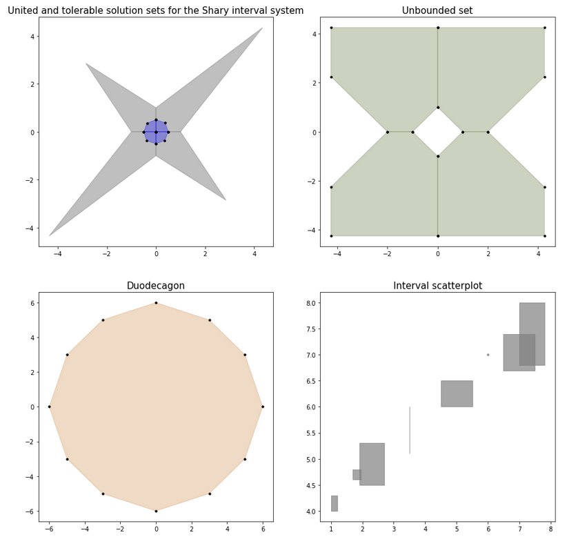
For a system of linear inequalities of the form ``A * x >= b`` or for an interval system of linear algebraic equations ``A * x = b``,
the solution sets are known to be polyhedral sets, convex or non-convex. We can visualize them and display all their vertices:
```python
import intvalpy as ip
ip.precision.extendedPrecisionQ = False
import numpy as np
iplt = ip.IPlot(figsize=(15, 15))
fig, ax = iplt.subplots(nrows=2, ncols=2)
#########################################################################
A, b = ip.Shary(2)
shary_uni = ip.IntLinIncR2(A, b, show=False)
shary_tol = ip.IntLinIncR2(A, b, consistency='tol', show=False)
axindex = (0, 0)
ax[axindex].set_title('United and tolerable solution sets for the Shary interval system')
ax[axindex].title.set_size(15)
iplt.IntLinIncR2(shary_uni, color='gray', alpha=0.5, s=0, axindex=axindex)
iplt.IntLinIncR2(shary_tol, color='blue', alpha=0.3, s=10, axindex=axindex)
#########################################################################
A = ip.Interval([
[[-1, 1], [-1, 1]],
[[-1, -1], [-1, 1]]
])
b = ip.Interval([[1, 1], [-2, 2]])
unconstrained_set = ip.IntLinIncR2(A, b, show=False)
axindex = (0, 1)
ax[axindex].set_title('Unbounded set')
ax[axindex].title.set_size(15)
iplt.IntLinIncR2(unconstrained_set, color='darkolivegreen', alpha=0.3, s=10, axindex=axindex)
#########################################################################
A = -np.array([[-3, -1],
[-2, -2],
[-1, -3],
[1, -3],
[2, -2],
[3, -1],
[3, 1],
[2, 2],
[1, 3],
[-1, 3],
[-2, 2],
[-3, 1]])
b = -np.array([18,16,18,18,16,18,18,16,18,18,16,18])
duodecagon = ip.lineqs(A, b, show=False)
axindex = (1, 0)
ax[axindex].set_title('Duodecagon')
ax[axindex].title.set_size(15)
iplt.lineqs(duodecagon, color='peru', alpha=0.3, s=10, axindex=axindex)
#########################################################################
x = ip.Interval([[1, 1.2], [1.9, 2.7], [1.7, 1.95], [3.5, 3.5],
[4.5, 5.5], [6, 6], [6.5, 7.5], [7, 7.8]])
y = ip.Interval([[4, 4.3], [4.5, 5.3], [4.6, 4.8], [5.1, 6],
[6, 6.5], [7, 7], [6.7, 7.4], [6.8, 8]])
axindex = (1, 1)
ax[axindex].set_title('Interval scatterplot')
ax[axindex].title.set_size(15)
iplt.scatter(x, y, color='gray', alpha=0.7, s=10, axindex=axindex)
```
It is also possible to make a three-dimensional (two-dimensional) slice of an N-dimensional figure and see what the set of solutions looks like
with fixed N-3 (N-2) parameters. A specific implementation of the algorithm can be found in the examples.
As a result, a gif image of the united set of solutions of the system proposed by S.P. Sharym is shown below, during the evolution of the 4th unknown.

### Recognizing functionals:
Before we start solving a system of equations with interval data it is necessary to understand whether it is solvable or not.
To do this we consider the problem of decidability recognition, i.e. non-emptiness of the set of solutions.
In the case of an interval linear (m x n)-system of equations, we will need to solve no more than 2\ :sup:`n`
linear inequalities of size 2m+n. This follows from the fact of convexity and polyhedra of the intersection of the sets of solutions
interval system of linear algebraic equations (ISLAE) with each of the orthants of **R**\ :sup:`n` space.
Reducing the number of inequalities is fundamentally impossible, which follows from the fact that the problem is intractable,
i.e. its NP-hardness. It is clear that the above described method is applicable only for small dimensionality of the problem,
that is why the *recognizing functional method* was proposed.
After global optimization, if the value of the functional is non-negative, then the system is solvable. If the value is negative,
then the set of parameters consistent with the data is empty, but the argument delivering the maximum of the functional minimizes this inconsistency.
As an example, it is proposed to investigate the Bart-Nuding system for the emptiness/non-emptiness of the tolerance set of solutions:
```python
import intvalpy as ip
# transition from extend precision (type mpf) to double precision (type float)
# ip.precision.extendedPrecisionQ = False
A = ip.Interval([
[[2, 4], [-2, 1]],
[[-1, 2], [2, 4]]
])
b = ip.Interval([[-2, 2], [-2, 2]])
tol = ip.linear.Tol.maximize(
A = A,
b = b,
x0 = None,
weight = None,
linear_constraint = None
)
print(tol)
```
### External decision evaluation:
To obtain an optimal external estimate of the united set of solutions of an interval system linear of algebraic equations (ISLAE),
a hybrid method of splitting PSS solutions is implemented. Since the task is NP-hard, the process can be stopped by the number of iterations completed.
PSS methods are consistently guaranteeing, i.e. when the process is interrupted at any number of iterations, an approximate estimate of the solution satisfies the required estimation method.
```python
import intvalpy as ip
# transition from extend precision (type mpf) to double precision (type float)
# ip.precision.extendedPrecisionQ = False
A, b = ip.Shary(12, N=12, alpha=0.23, beta=0.35)
pss = ip.linear.PSS(A, b)
print('pss: ', pss)
```
### Interval system of nonlinear equations:
For nonlinear systems, the simplest multidimensional interval methods of Krawczyk and Hansen-Sengupta are implemented for solving nonlinear systems:
```python
import intvalpy as ip
# transition from extend precision (type mpf) to double precision (type float)
# ip.precision.extendedPrecisionQ = False
epsilon = 0.1
def f(x):
return ip.asinterval([x[0]**2 + x[1]**2 - 1 - ip.Interval(-epsilon, epsilon),
x[0] - x[1]**2])
def J(x):
result = [[2*x[0], 2*x[1]],
[1, -2*x[1]]]
return ip.asinterval(result)
ip.nonlinear.HansenSengupta(f, J, ip.Interval([0.5,0.5],[1,1]))
```
The library also provides the simplest interval global optimization:
```python
import intvalpy as ip
# transition from extend precision (type mpf) to double precision (type float)
# ip.precision.extendedPrecisionQ = False
def levy(x):
z = 1 + (x - 1) / 4
t1 = np.sin( np.pi * z[0] )**2
t2 = sum(((x - 1) ** 2 * (1 + 10 * np.sin(np.pi * x + 1) ** 2))[:-1])
t3 = (z[-1] - 1) ** 2 * (1 + np.sin(2*np.pi * z[-1]) ** 2)
return t1 + t2 + t3
N = 2
x = ip.Interval([-5]*N, [5]*N)
ip.nonlinear.globopt(levy, x, tol=1e-14)
```
Links
-----
* [Article](<https://www.researchgate.net/publication/371587916_IntvalPy_-_a_Python_Interval_Computation_Library>)
* [Homepage](<https://github.com/AndrosovAS/intvalpy>)
* [Online documentation](<https://intvalpy.readthedocs.io/ru/latest/#>)
* [PyPI package](<https://pypi.org/project/intvalpy/>)
* A detailed [monograph](<http://www.nsc.ru/interval/Library/InteBooks/SharyBook.pdf>) on interval theory
Raw data
{
"_id": null,
"home_page": "https://github.com/AndrosovAS/intvalpy",
"name": "intvalpy",
"maintainer": "",
"docs_url": null,
"requires_python": "",
"maintainer_email": "",
"keywords": "Interval,inequality visualization,optimal solutions,math,range",
"author": "\u0410\u043d\u0434\u0440\u043e\u0441\u043e\u0432 \u0410\u0440\u0442\u0435\u043c \u0421\u0442\u0430\u043d\u0438\u0441\u043b\u0430\u0432\u043e\u0432\u0438\u0447, \u0428\u0430\u0440\u044b\u0439 \u0421\u0435\u0440\u0433\u0435\u0439 \u041f\u0435\u0442\u0440\u043e\u0432\u0438\u0447",
"author_email": "artem.androsov@gmail.com, shary@ict.nsc.ru",
"download_url": "https://files.pythonhosted.org/packages/e7/bd/25a9c9c25e059dd845018f0b70dbcd2c5c154afa636552ebc5d8841c74a5/intvalpy-1.6.1.tar.gz",
"platform": null,
"description": "# Interval library in Python\r\n\r\nThe Python module implements an algebraically closed interval arithmetic for interval computations, solving interval systems of both\r\nlinear and nonlinear equations, and visualizing solution sets for interval systems of equations.\r\n\r\nFor details, see the complete documentation on [API](https://intvalpy.readthedocs.io/ru/latest/index.html).\r\n\r\n## Installation\r\n\r\nMake sure you have all the system-wide dependencies, then install the module itself:\r\n```\r\npip install intvalpy\r\n```\r\n\r\n## Examples\r\n\r\n### Visualizing solution sets\r\n\r\nFor a system of linear inequalities of the form ``A * x >= b`` or for an interval system of linear algebraic equations ``A * x = b``,\r\nthe solution sets are known to be polyhedral sets, convex or non-convex. We can visualize them and display all their vertices:\r\n\r\n```python\r\nimport intvalpy as ip\r\nip.precision.extendedPrecisionQ = False\r\nimport numpy as np\r\n\r\n\r\niplt = ip.IPlot(figsize=(15, 15))\r\nfig, ax = iplt.subplots(nrows=2, ncols=2)\r\n\r\n\r\n#########################################################################\r\nA, b = ip.Shary(2)\r\nshary_uni = ip.IntLinIncR2(A, b, show=False)\r\nshary_tol = ip.IntLinIncR2(A, b, consistency='tol', show=False)\r\n\r\naxindex = (0, 0)\r\nax[axindex].set_title('United and tolerable solution sets for the Shary interval system')\r\nax[axindex].title.set_size(15)\r\niplt.IntLinIncR2(shary_uni, color='gray', alpha=0.5, s=0, axindex=axindex)\r\niplt.IntLinIncR2(shary_tol, color='blue', alpha=0.3, s=10, axindex=axindex)\r\n\r\n#########################################################################\r\nA = ip.Interval([\r\n [[-1, 1], [-1, 1]],\r\n [[-1, -1], [-1, 1]]\r\n])\r\nb = ip.Interval([[1, 1], [-2, 2]])\r\nunconstrained_set = ip.IntLinIncR2(A, b, show=False)\r\n\r\naxindex = (0, 1)\r\nax[axindex].set_title('Unbounded set')\r\nax[axindex].title.set_size(15)\r\niplt.IntLinIncR2(unconstrained_set, color='darkolivegreen', alpha=0.3, s=10, axindex=axindex)\r\n\r\n#########################################################################\r\nA = -np.array([[-3, -1],\r\n [-2, -2],\r\n [-1, -3],\r\n [1, -3],\r\n [2, -2],\r\n [3, -1],\r\n [3, 1],\r\n [2, 2],\r\n [1, 3],\r\n [-1, 3],\r\n [-2, 2],\r\n [-3, 1]])\r\nb = -np.array([18,16,18,18,16,18,18,16,18,18,16,18])\r\nduodecagon = ip.lineqs(A, b, show=False)\r\n\r\naxindex = (1, 0)\r\nax[axindex].set_title('Duodecagon')\r\nax[axindex].title.set_size(15)\r\niplt.lineqs(duodecagon, color='peru', alpha=0.3, s=10, axindex=axindex)\r\n\r\n#########################################################################\r\nx = ip.Interval([[1, 1.2], [1.9, 2.7], [1.7, 1.95], [3.5, 3.5],\r\n [4.5, 5.5], [6, 6], [6.5, 7.5], [7, 7.8]])\r\ny = ip.Interval([[4, 4.3], [4.5, 5.3], [4.6, 4.8], [5.1, 6],\r\n [6, 6.5], [7, 7], [6.7, 7.4], [6.8, 8]])\r\n\r\naxindex = (1, 1)\r\nax[axindex].set_title('Interval scatterplot')\r\nax[axindex].title.set_size(15)\r\niplt.scatter(x, y, color='gray', alpha=0.7, s=10, axindex=axindex)\r\n```\r\n\r\n\r\nIt is also possible to make a three-dimensional (two-dimensional) slice of an N-dimensional figure and see what the set of solutions looks like\r\nwith fixed N-3 (N-2) parameters. A specific implementation of the algorithm can be found in the examples.\r\nAs a result, a gif image of the united set of solutions of the system proposed by S.P. Sharym is shown below, during the evolution of the 4th unknown.\r\n\r\n\r\n\r\n### Recognizing functionals:\r\n\r\nBefore we start solving a system of equations with interval data it is necessary to understand whether it is solvable or not.\r\nTo do this we consider the problem of decidability recognition, i.e. non-emptiness of the set of solutions.\r\nIn the case of an interval linear (m x n)-system of equations, we will need to solve no more than 2\\ :sup:`n`\r\nlinear inequalities of size 2m+n. This follows from the fact of convexity and polyhedra of the intersection of the sets of solutions\r\ninterval system of linear algebraic equations (ISLAE) with each of the orthants of **R**\\ :sup:`n` space.\r\nReducing the number of inequalities is fundamentally impossible, which follows from the fact that the problem is intractable,\r\ni.e. its NP-hardness. It is clear that the above described method is applicable only for small dimensionality of the problem,\r\nthat is why the *recognizing functional method* was proposed.\r\n\r\nAfter global optimization, if the value of the functional is non-negative, then the system is solvable. If the value is negative,\r\nthen the set of parameters consistent with the data is empty, but the argument delivering the maximum of the functional minimizes this inconsistency.\r\n\r\nAs an example, it is proposed to investigate the Bart-Nuding system for the emptiness/non-emptiness of the tolerance set of solutions:\r\n\r\n```python\r\nimport intvalpy as ip\r\n# transition from extend precision (type mpf) to double precision (type float)\r\n# ip.precision.extendedPrecisionQ = False\r\n\r\nA = ip.Interval([\r\n [[2, 4], [-2, 1]],\r\n [[-1, 2], [2, 4]]\r\n])\r\nb = ip.Interval([[-2, 2], [-2, 2]])\r\n\r\ntol = ip.linear.Tol.maximize(\r\n A = A, \r\n b = b,\r\n x0 = None,\r\n weight = None,\r\n linear_constraint = None\r\n)\r\nprint(tol)\r\n```\r\n\r\n### External decision evaluation:\r\n\r\nTo obtain an optimal external estimate of the united set of solutions of an interval system linear of algebraic equations (ISLAE),\r\na hybrid method of splitting PSS solutions is implemented. Since the task is NP-hard, the process can be stopped by the number of iterations completed.\r\nPSS methods are consistently guaranteeing, i.e. when the process is interrupted at any number of iterations, an approximate estimate of the solution satisfies the required estimation method.\r\n\r\n```python\r\nimport intvalpy as ip\r\n# transition from extend precision (type mpf) to double precision (type float)\r\n# ip.precision.extendedPrecisionQ = False\r\n\r\nA, b = ip.Shary(12, N=12, alpha=0.23, beta=0.35)\r\npss = ip.linear.PSS(A, b)\r\nprint('pss: ', pss)\r\n```\r\n\r\n### Interval system of nonlinear equations:\r\n\r\nFor nonlinear systems, the simplest multidimensional interval methods of Krawczyk and Hansen-Sengupta are implemented for solving nonlinear systems:\r\n\r\n```python\r\nimport intvalpy as ip\r\n# transition from extend precision (type mpf) to double precision (type float)\r\n# ip.precision.extendedPrecisionQ = False\r\n\r\nepsilon = 0.1\r\ndef f(x):\r\n return ip.asinterval([x[0]**2 + x[1]**2 - 1 - ip.Interval(-epsilon, epsilon),\r\n x[0] - x[1]**2])\r\n\r\ndef J(x): \r\n result = [[2*x[0], 2*x[1]],\r\n [1, -2*x[1]]]\r\n return ip.asinterval(result)\r\n\r\nip.nonlinear.HansenSengupta(f, J, ip.Interval([0.5,0.5],[1,1]))\r\n```\r\n\r\nThe library also provides the simplest interval global optimization:\r\n\r\n```python\r\nimport intvalpy as ip\r\n# transition from extend precision (type mpf) to double precision (type float)\r\n# ip.precision.extendedPrecisionQ = False\r\n\r\ndef levy(x):\r\n z = 1 + (x - 1) / 4\r\n t1 = np.sin( np.pi * z[0] )**2\r\n t2 = sum(((x - 1) ** 2 * (1 + 10 * np.sin(np.pi * x + 1) ** 2))[:-1])\r\n t3 = (z[-1] - 1) ** 2 * (1 + np.sin(2*np.pi * z[-1]) ** 2)\r\n return t1 + t2 + t3\r\n\r\nN = 2\r\nx = ip.Interval([-5]*N, [5]*N)\r\nip.nonlinear.globopt(levy, x, tol=1e-14)\r\n```\r\n\r\nLinks\r\n-----\r\n\r\n* [Article](<https://www.researchgate.net/publication/371587916_IntvalPy_-_a_Python_Interval_Computation_Library>)\r\n\r\n* [Homepage](<https://github.com/AndrosovAS/intvalpy>)\r\n\r\n* [Online documentation](<https://intvalpy.readthedocs.io/ru/latest/#>)\r\n\r\n* [PyPI package](<https://pypi.org/project/intvalpy/>)\r\n\r\n* A detailed [monograph](<http://www.nsc.ru/interval/Library/InteBooks/SharyBook.pdf>) on interval theory\r\n",
"bugtrack_url": null,
"license": "MIT License",
"summary": "IntvalPy - a Python interval computation library",
"version": "1.6.1",
"project_urls": {
"Homepage": "https://github.com/AndrosovAS/intvalpy"
},
"split_keywords": [
"interval",
"inequality visualization",
"optimal solutions",
"math",
"range"
],
"urls": [
{
"comment_text": "",
"digests": {
"blake2b_256": "e7bd25a9c9c25e059dd845018f0b70dbcd2c5c154afa636552ebc5d8841c74a5",
"md5": "8cb645a19eb5dc499b2f3f51dce872f5",
"sha256": "f9ba70a359013fd8c20becac57ec9af854335e50185e9f42b75cecc07157c308"
},
"downloads": -1,
"filename": "intvalpy-1.6.1.tar.gz",
"has_sig": false,
"md5_digest": "8cb645a19eb5dc499b2f3f51dce872f5",
"packagetype": "sdist",
"python_version": "source",
"requires_python": null,
"size": 39742,
"upload_time": "2024-02-17T14:56:18",
"upload_time_iso_8601": "2024-02-17T14:56:18.253877Z",
"url": "https://files.pythonhosted.org/packages/e7/bd/25a9c9c25e059dd845018f0b70dbcd2c5c154afa636552ebc5d8841c74a5/intvalpy-1.6.1.tar.gz",
"yanked": false,
"yanked_reason": null
}
],
"upload_time": "2024-02-17 14:56:18",
"github": true,
"gitlab": false,
"bitbucket": false,
"codeberg": false,
"github_user": "AndrosovAS",
"github_project": "intvalpy",
"travis_ci": true,
"coveralls": false,
"github_actions": false,
"lcname": "intvalpy"
}


