# REMclust
---
### Introduction
REMclust is a Python package for model-based clustering based on Gaussian mixture models. It uses a peak finding criterion to find modes within the data set. An initial mode set is taken to be the means in Gaussian components.
Once the initial mode set has been selected, an iterative procedure comprising two blocks is triggered. A mixture is produced for each iteration.
1. An EM block to fit the covariances and mixing proportions of the components
2. A pruning block to remove one of the components as part of an efficient model selection strategy.
Additional functionalities are available for displaying and visualising fitted models and clustering results.
---
### Data
The data set used in this vignette is the [Palmer Archipelago (Antarctica) Penguin Data](https://github.com/allisonhorst/palmerpenguins). In this particular data set, the features are measured across different scales, for example, culmen depth ranges from 13.1 to 21.5, while body mass ranges from 2700 to 6300. This difference in scale can negatively impact the clustering accuracy, so standardisation was performed. Standardisation ensures that all features are measured in comparable scales and is the process that is recommended when the data set that is being clustered has features that vary widely in scale. The following methods are used to load the dataset.
```python
import numpy as np
from sklearn import preprocessing
from REMclust import REM
```
```python
data = np.genfromtxt('Data/penguin.csv', delimiter=",")
x = data[:,1:]
y = data[:, 0]
labels = ['Culmen Length', 'Culmen Depth', 'Flipper Length', 'Body Mass', 'Delta 15 N (o/oo)', 'Delta 13 C (o/oo)']
x = x[1:,:]
scaler = preprocessing.StandardScaler().fit(x)
x = scaler.transform(x)
n_samples, n_features = x.shape
```
---
### Initialisation
The first step in applying REM to the data set is to initialise an REM object.
```python
REM(data, covariance_type='full', criteria='all', bandwidth='diagonal', tol=1e-3, reg_covar=1e-6, max_iter=100)
```
- **data (array-like of shape (n_samples, n_features))**: The data the model is being fitted to.
- **covariance_type {'full', 'tied', 'diag', 'spherical'}**: A string describing the type of covariance parameters to use. full: each component has its own general covariance matrix. tied: all components share the same general covariance matrix. diag: each component has its own diagonal covariance matrix. spherical: each component has its own single variance.
- **criteria {'all', 'aic', 'bic', 'icl'}**: A string defining the criterion score used in model selection. At the end of each iteration of REM, a mixture is produced. The mixture that minimises this score will be taken as the optimal clustering.
- **bandwidth ({'diagonal', 'spherical', 'normal_reference'}, int, float)**: Either a string, integer, or floating point number that defines the bandwidth used when finding the modes.
- **tol (float)**: The convergence threshold. EM iterations will stop when the lower bound average gain is below this threshold.
- **reg_covar (float)**: Non-negative regularisation added to the diagonal of covariance. Allows to ensure that the covariance matrices are all positive.
- **max_iter (int)**: The number of EM iterations to perform.
```python
bndwk = int(np.floor(np.min((30, np.log(n_samples)))))
cluster = REM(data=x, covariance_type="full", criteria="icl",bandwidth=bndwk, tol=1e-4)
```
### Mode Selection
The user must select the initial mode set. To do this, they must select a *distance_threshold* and *density_threshold*. To aid in this, the method
```python
REM.mode_decision_plot()
```
is provided. This method draws two plots. One is a plot of the distance between a point to its nearest neighbour with a higher density against the points' density. This plot will allow the user to select the appropriate thresholds. The ideal modes have both a high distance and density. The second plot shows the product of the distance and the density for each point, allowing the user to determine the likely number of modes easily.
```python
cluster.mode_decision_plot()
```

REMclust also provides the method:
```python
REM.kde_contour_plot(dimensions=None, axis_labels=None)
```
- **dimensions (list(int))**: A list of integers that defines the features that will be plotted. If left as None, all features will be plotted.
- **axis_labels (list(str))**: A list of strings that define the labels for the axes.
This method provides a contour plot of the estimated KDE densities.
```python
cluster.kde_contour_plot(dimensions=[1, 2, 4, 5], axis_labels=[labels[1], labels[2], labels[4], labels[5]])
```

### Clustering
To perform clustering, the following method is run:
```python
fit(max_components=5, density_threshold=None, distance_threshold=None)
```
- **max_components (int)**: An integer that defines the initial size of the mode set. The modes with the highest $density \times distance$ will fill the set.
- **density_threshold (float)**: A float defining the mode's density threshold. A mode must have a higher density to be included in the initial mode set.
- **distance_threshold (float)**: A float defining the mode's distance threshold. A mode must have a higher distance to be included in the initial mode set.
**Note:** There are two possible ways to define the mode set:
1. Setting the max components value k, in which the k modes with the highest $density \times distance$ will be included in the initial mode set.
2. Setting the two thresholds will include the modes exceeding both in the initial mode set.
Should the user set the max components and the thresholds, the mode set created by the thresholds will be preferred.
```python
cluster.fit(density_threshold = 1.6, distance_threshold = 3)
```
---
### Visualisation
REMclust provides visualisation tools that allow the user to explore the clustering results. The first of these is:
```python
REM.classification_plot(mixture_selection='', dimensions=None, axis_labels=None)
```
A plot of the classification of the data on which the clustering was performed.
- **mixture_selection {'', 'aic', bic', 'icl'}** This defines whether the user would like to plot the results from the model selected by AIC, BIC, or ICL. This is required if the initial criterion was set to 'all'. Otherwise, it should not be set.
- **dimensions (list(int))**: A list of integers that defines the features that will be plotted. If left as None all features will be plotted.
- **axis_labels (list(str))**: A list of strings that define the labels for the axes.
```python
cluster.classification_plot(dimensions=[0,1,2], axis_labels=[labels[0], labels[1], labels[2]])
```

Another visualisation method provided by REMclust is:
```python
REM.uncertainty_plot(mixture_selection='', dimensions=None, axis_labels=None)
```
A plot of the uncertainty of the data that the clustering was performed on. Uncertainty is measured as the inverse of the difference between the probability that a point belongs to the assigned cluster and the probability that it belongs to the next most likely cluster. The uncertainty score for a point is represented by its size in the scatter plot
- **mixture_selection {'', 'aic', bic', 'icl'}** This defines whether the user would like to plot the results from the model selected by AIC, BIC, or ICL. This is required if the initial criterion was set to 'all'. Otherwise, it should not be set.
- **dimensions (list(int))**: A list of integers that defines the features that will be plotted. If left as None all features will be plotted.
- **axis_labels (list(str))**: A list of strings that define the labels for the axes.
```python
cluster.uncertainty_plot()
```

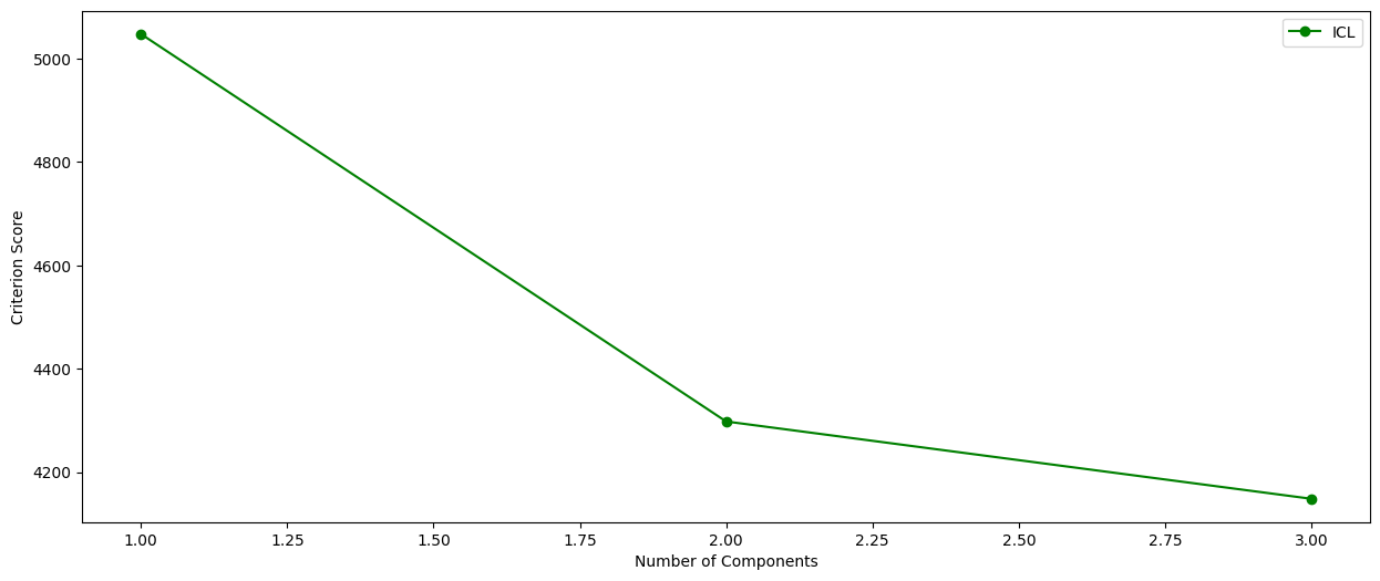
Finally, REMclust provides:
```python
REM.criterion_plot()
```
A plot of the criterion scores for the different models fit
```python
cluster.criterion_plot()
```
### Summary
As well as visualisations, REMclust also provides a method that prints text-based summaries of the clustering results.
```python
REM.summary(parameters=False, classification=False, criterion_scores=False)
```
- **parameters (boolean)**: If TRUE, the parameters of mixture components are printed.
- **classification (boolean)**: If TRUE, a table of classifications/clustering of observations is printed.
- **criterion_scores (boolean)**: If TRUE, all the tested models' criterion scores are printed.
```python
cluster.summary(parameters=True, classification=True, criterion_scores=True)
```
ICL scores:
Number of components ICL
1 5047.430917914943
2 4297.94941510035
3 4148.377773911351
REM full model with 3 components.
Log-Likelihood n ICL
-5.557734230801972 330 5047.430917914943
Clustering Table:
0 1 2
142 66 122
Mixing proportions:
0 1 2
0.4298003096720814 0.20016916200970244 0.37003052831821626
Means:
[,0] [,1] [,2] [,3] [,4] [,5]
[0,] -1.4428802310212794 0.09847251687109626 -1.0265979344127258 -1.1391980159992219 0.3155521383966185 -0.7729366056647325
[1,] 1.3519480199837914 0.9589566596231957 -0.02238822512058244 -0.3306680319415391 1.2786263024434288 1.6899270286191586
[2,] 0.6348539292653853 -1.5718790543535683 0.7666336893232445 0.8199323299867016 -1.1008070686917295 -0.6913133901121228
Variances:
[0,,]
[,0] [,1] [,2] [,3] [,4] [,5]
[0,] 0.4822812184430567 0.3738893956467974 0.193523105176551 0.40423726432377793 -0.003501864571959848 0.329894630536289
[1,] 0.3738893956467974 0.6550574932653658 0.21753500797095157 0.4741998306014431 -0.00992735456677892 0.3937308037948014
[2,] 0.19352310517655102 0.21753500797095157 0.2718029819739479 0.2468028741147682 -0.04353334076528556 0.050373041668713446
[3,] 0.40423726432377804 0.4741998306014431 0.24680287411476814 0.5804133660047892 -0.04564674250026045 0.3120111725984246
[4,] -0.003501864571959848 -0.00992735456677892 -0.04353334076528556 -0.04564674250026045 0.605721076965007 0.24359100999515984
[5,] 0.329894630536289 0.39373080379480146 0.05037304166871344 0.3120111725984246 0.2435910099951599 0.9734990100580053
[1,,]
[,0] [,1] [,2] [,3] [,4] [,5]
[0,] 0.6030243673968754 0.36971785590641787 0.3180714184444992 0.2819457120118386 0.13972172089522267 0.14283451171713746
[1,] 0.36971785590641787 0.42031932795360744 0.2774602915474537 0.2492296460273077 0.0896044343842434 0.09098707945986677
[2,] 0.3180714184444992 0.2774602915474537 0.3948606216756481 0.26022526338261737 0.15322162166230058 0.1130208353320999
[3,] 0.2819457120118386 0.24922964602730777 0.26022526338261737 0.3080550789154811 0.03108846196186896 0.07151058239485042
[4,] 0.13972172089522264 0.08960443438424338 0.1532216216623006 0.031088461961868954 0.4724004958694611 0.008903299028650682
[5,] 0.14283451171713746 0.09098707945986678 0.11302083533209989 0.07151058239485043 0.008903299028650669 0.14296027583057802
[2,,]
[,0] [,1] [,2] [,3] [,4] [,5]
[0,] 0.3237502041668178 0.1832232100008559 0.17627326183722639 0.24011283063151295 0.039792481708646285 0.008945551681238563
[1,] 0.1832232100008559 0.4963399760152181 0.3486971318082281 0.34961971873551334 0.15621370324790285 0.007855296319765621
[2,] 0.17627326183722639 0.3486971318082281 0.35462935635233916 0.298456233903807 0.14700826635676648 -0.006249823224869592
[3,] 0.24011283063151295 0.34961971873551334 0.298456233903807 0.45821934107892376 0.09832322755784137 0.052332556416111606
[4,] 0.039792481708646285 0.15621370324790287 0.14700826635676648 0.09832322755784138 0.2770290751477198 -0.17808975073244143
[5,] 0.008945551681238567 0.007855296319765621 -0.0062498232248696 0.052332556416111606 -0.17808975073244143 0.47245403005359093
Raw data
{
"_id": null,
"home_page": "https://github.com/r-swords/REMclust",
"name": "REMclust",
"maintainer": "",
"docs_url": null,
"requires_python": "",
"maintainer_email": "",
"keywords": "REM,Reinforced EM,Clustering,Density-Based Clustering,Parametric Density-Based Clustering,Gaussian Mixture Models",
"author": "Joshua Tobin, Ralph Swords, Mimi Zhang",
"author_email": "tobinjo@tcd.ie",
"download_url": "https://files.pythonhosted.org/packages/f3/b8/8d76daed087f81cc1c63b18bcac481eb5eec1ead3dd893090faeacf30585/REMclust-1.2.tar.gz",
"platform": null,
"description": "# REMclust\r\n---\r\n### Introduction\r\n\r\nREMclust is a Python package for model-based clustering based on Gaussian mixture models. It uses a peak finding criterion to find modes within the data set. An initial mode set is taken to be the means in Gaussian components.\r\n\r\nOnce the initial mode set has been selected, an iterative procedure comprising two blocks is triggered. A mixture is produced for each iteration.\r\n1. An EM block to fit the covariances and mixing proportions of the components\r\n2. A pruning block to remove one of the components as part of an efficient model selection strategy.\r\n\r\nAdditional functionalities are available for displaying and visualising fitted models and clustering results.\r\n\r\n---\r\n### Data\r\n\r\nThe data set used in this vignette is the [Palmer Archipelago (Antarctica) Penguin Data](https://github.com/allisonhorst/palmerpenguins). In this particular data set, the features are measured across different scales, for example, culmen depth ranges from 13.1 to 21.5, while body mass ranges from 2700 to 6300. This difference in scale can negatively impact the clustering accuracy, so standardisation was performed. Standardisation ensures that all features are measured in comparable scales and is the process that is recommended when the data set that is being clustered has features that vary widely in scale. The following methods are used to load the dataset.\r\n\r\n\r\n```python\r\nimport numpy as np\r\nfrom sklearn import preprocessing\r\n\r\nfrom REMclust import REM\r\n```\r\n\r\n\r\n```python\r\ndata = np.genfromtxt('Data/penguin.csv', delimiter=\",\")\r\nx = data[:,1:]\r\ny = data[:, 0]\r\nlabels = ['Culmen Length', 'Culmen Depth', 'Flipper Length', 'Body Mass', 'Delta 15 N (o/oo)', 'Delta 13 C (o/oo)']\r\nx = x[1:,:]\r\nscaler = preprocessing.StandardScaler().fit(x)\r\nx = scaler.transform(x)\r\n\r\nn_samples, n_features = x.shape\r\n```\r\n\r\n---\r\n### Initialisation\r\nThe first step in applying REM to the data set is to initialise an REM object.\r\n```python\r\nREM(data, covariance_type='full', criteria='all', bandwidth='diagonal', tol=1e-3, reg_covar=1e-6, max_iter=100)\r\n```\r\n- **data (array-like of shape (n_samples, n_features))**: The data the model is being fitted to.\r\n- **covariance_type {'full', 'tied', 'diag', 'spherical'}**: A string describing the type of covariance parameters to use. full: each component has its own general covariance matrix. tied: all components share the same general covariance matrix. diag: each component has its own diagonal covariance matrix. spherical: each component has its own single variance.\r\n- **criteria {'all', 'aic', 'bic', 'icl'}**: A string defining the criterion score used in model selection. At the end of each iteration of REM, a mixture is produced. The mixture that minimises this score will be taken as the optimal clustering.\r\n- **bandwidth ({'diagonal', 'spherical', 'normal_reference'}, int, float)**: Either a string, integer, or floating point number that defines the bandwidth used when finding the modes.\r\n- **tol (float)**: The convergence threshold. EM iterations will stop when the lower bound average gain is below this threshold.\r\n- **reg_covar (float)**: Non-negative regularisation added to the diagonal of covariance. Allows to ensure that the covariance matrices are all positive.\r\n- **max_iter (int)**: The number of EM iterations to perform.\r\n\r\n\r\n```python\r\nbndwk = int(np.floor(np.min((30, np.log(n_samples)))))\r\ncluster = REM(data=x, covariance_type=\"full\", criteria=\"icl\",bandwidth=bndwk, tol=1e-4)\r\n```\r\n\r\n### Mode Selection\r\n\r\nThe user must select the initial mode set. To do this, they must select a *distance_threshold* and *density_threshold*. To aid in this, the method\r\n```python\r\nREM.mode_decision_plot()\r\n```\r\nis provided. This method draws two plots. One is a plot of the distance between a point to its nearest neighbour with a higher density against the points' density. This plot will allow the user to select the appropriate thresholds. The ideal modes have both a high distance and density. The second plot shows the product of the distance and the density for each point, allowing the user to determine the likely number of modes easily.\r\n\r\n\r\n```python\r\ncluster.mode_decision_plot()\r\n```\r\n\r\n\r\n \r\n\r\n\r\nREMclust also provides the method:\r\n```python\r\nREM.kde_contour_plot(dimensions=None, axis_labels=None)\r\n```\r\n- **dimensions (list(int))**: A list of integers that defines the features that will be plotted. If left as None, all features will be plotted.\r\n- **axis_labels (list(str))**: A list of strings that define the labels for the axes.\r\n\r\nThis method provides a contour plot of the estimated KDE densities.\r\n\r\n\r\n```python\r\ncluster.kde_contour_plot(dimensions=[1, 2, 4, 5], axis_labels=[labels[1], labels[2], labels[4], labels[5]])\r\n```\r\n\r\n\r\n \r\n\r\n \r\n\r\n\r\n### Clustering\r\n\r\nTo perform clustering, the following method is run:\r\n```python\r\nfit(max_components=5, density_threshold=None, distance_threshold=None)\r\n```\r\n- **max_components (int)**: An integer that defines the initial size of the mode set. The modes with the highest $density \\times distance$ will fill the set.\r\n- **density_threshold (float)**: A float defining the mode's density threshold. A mode must have a higher density to be included in the initial mode set.\r\n- **distance_threshold (float)**: A float defining the mode's distance threshold. A mode must have a higher distance to be included in the initial mode set.\r\n\r\n**Note:** There are two possible ways to define the mode set:\r\n1. Setting the max components value k, in which the k modes with the highest $density \\times distance$ will be included in the initial mode set.\r\n2. Setting the two thresholds will include the modes exceeding both in the initial mode set.\r\n\r\nShould the user set the max components and the thresholds, the mode set created by the thresholds will be preferred.\r\n\r\n\r\n```python\r\ncluster.fit(density_threshold = 1.6, distance_threshold = 3)\r\n```\r\n\r\n---\r\n\r\n\r\n### Visualisation\r\n\r\nREMclust provides visualisation tools that allow the user to explore the clustering results. The first of these is:\r\n```python\r\nREM.classification_plot(mixture_selection='', dimensions=None, axis_labels=None)\r\n```\r\nA plot of the classification of the data on which the clustering was performed.\r\n- **mixture_selection {'', 'aic', bic', 'icl'}** This defines whether the user would like to plot the results from the model selected by AIC, BIC, or ICL. This is required if the initial criterion was set to 'all'. Otherwise, it should not be set.\r\n- **dimensions (list(int))**: A list of integers that defines the features that will be plotted. If left as None all features will be plotted.\r\n- **axis_labels (list(str))**: A list of strings that define the labels for the axes.\r\n\r\n\r\n```python\r\ncluster.classification_plot(dimensions=[0,1,2], axis_labels=[labels[0], labels[1], labels[2]])\r\n```\r\n\r\n\r\n \r\n\r\n \r\n\r\n\r\nAnother visualisation method provided by REMclust is:\r\n```python\r\nREM.uncertainty_plot(mixture_selection='', dimensions=None, axis_labels=None)\r\n```\r\nA plot of the uncertainty of the data that the clustering was performed on. Uncertainty is measured as the inverse of the difference between the probability that a point belongs to the assigned cluster and the probability that it belongs to the next most likely cluster. The uncertainty score for a point is represented by its size in the scatter plot\r\n- **mixture_selection {'', 'aic', bic', 'icl'}** This defines whether the user would like to plot the results from the model selected by AIC, BIC, or ICL. This is required if the initial criterion was set to 'all'. Otherwise, it should not be set.\r\n- **dimensions (list(int))**: A list of integers that defines the features that will be plotted. If left as None all features will be plotted.\r\n- **axis_labels (list(str))**: A list of strings that define the labels for the axes.\r\n\r\n\r\n```python\r\ncluster.uncertainty_plot()\r\n```\r\n\r\n\r\n \r\n\r\n \r\n\r\n\r\nFinally, REMclust provides:\r\n```python\r\nREM.criterion_plot()\r\n```\r\nA plot of the criterion scores for the different models fit\r\n\r\n\r\n```python\r\ncluster.criterion_plot()\r\n```\r\n\r\n\r\n \r\n\r\n \r\n\r\n\r\n### Summary\r\nAs well as visualisations, REMclust also provides a method that prints text-based summaries of the clustering results.\r\n```python\r\nREM.summary(parameters=False, classification=False, criterion_scores=False)\r\n```\r\n- **parameters (boolean)**: If TRUE, the parameters of mixture components are printed.\r\n- **classification (boolean)**: If TRUE, a table of classifications/clustering of observations is printed.\r\n- **criterion_scores (boolean)**: If TRUE, all the tested models' criterion scores are printed.\r\n\r\n\r\n```python\r\ncluster.summary(parameters=True, classification=True, criterion_scores=True)\r\n```\r\n\r\n ICL scores:\r\n Number of components ICL \r\n 1 5047.430917914943\r\n 2 4297.94941510035\r\n 3 4148.377773911351\r\n \r\n REM full model with 3 components.\r\n \r\n Log-Likelihood n ICL \r\n -5.557734230801972 330 5047.430917914943\r\n \r\n Clustering Table:\r\n 0 1 2\r\n 142 66 122\r\n \r\n Mixing proportions:\r\n 0 1 2\r\n 0.4298003096720814 0.20016916200970244 0.37003052831821626\r\n \r\n Means:\r\n [,0] [,1] [,2] [,3] [,4] [,5]\r\n [0,] -1.4428802310212794 0.09847251687109626 -1.0265979344127258 -1.1391980159992219 0.3155521383966185 -0.7729366056647325\r\n [1,] 1.3519480199837914 0.9589566596231957 -0.02238822512058244 -0.3306680319415391 1.2786263024434288 1.6899270286191586\r\n [2,] 0.6348539292653853 -1.5718790543535683 0.7666336893232445 0.8199323299867016 -1.1008070686917295 -0.6913133901121228\r\n \r\n Variances:\r\n [0,,]\r\n [,0] [,1] [,2] [,3] [,4] [,5]\r\n [0,] 0.4822812184430567 0.3738893956467974 0.193523105176551 0.40423726432377793 -0.003501864571959848 0.329894630536289\r\n [1,] 0.3738893956467974 0.6550574932653658 0.21753500797095157 0.4741998306014431 -0.00992735456677892 0.3937308037948014\r\n [2,] 0.19352310517655102 0.21753500797095157 0.2718029819739479 0.2468028741147682 -0.04353334076528556 0.050373041668713446\r\n [3,] 0.40423726432377804 0.4741998306014431 0.24680287411476814 0.5804133660047892 -0.04564674250026045 0.3120111725984246\r\n [4,] -0.003501864571959848 -0.00992735456677892 -0.04353334076528556 -0.04564674250026045 0.605721076965007 0.24359100999515984\r\n [5,] 0.329894630536289 0.39373080379480146 0.05037304166871344 0.3120111725984246 0.2435910099951599 0.9734990100580053\r\n [1,,]\r\n [,0] [,1] [,2] [,3] [,4] [,5]\r\n [0,] 0.6030243673968754 0.36971785590641787 0.3180714184444992 0.2819457120118386 0.13972172089522267 0.14283451171713746\r\n [1,] 0.36971785590641787 0.42031932795360744 0.2774602915474537 0.2492296460273077 0.0896044343842434 0.09098707945986677\r\n [2,] 0.3180714184444992 0.2774602915474537 0.3948606216756481 0.26022526338261737 0.15322162166230058 0.1130208353320999\r\n [3,] 0.2819457120118386 0.24922964602730777 0.26022526338261737 0.3080550789154811 0.03108846196186896 0.07151058239485042\r\n [4,] 0.13972172089522264 0.08960443438424338 0.1532216216623006 0.031088461961868954 0.4724004958694611 0.008903299028650682\r\n [5,] 0.14283451171713746 0.09098707945986678 0.11302083533209989 0.07151058239485043 0.008903299028650669 0.14296027583057802\r\n [2,,]\r\n [,0] [,1] [,2] [,3] [,4] [,5]\r\n [0,] 0.3237502041668178 0.1832232100008559 0.17627326183722639 0.24011283063151295 0.039792481708646285 0.008945551681238563\r\n [1,] 0.1832232100008559 0.4963399760152181 0.3486971318082281 0.34961971873551334 0.15621370324790285 0.007855296319765621\r\n [2,] 0.17627326183722639 0.3486971318082281 0.35462935635233916 0.298456233903807 0.14700826635676648 -0.006249823224869592\r\n [3,] 0.24011283063151295 0.34961971873551334 0.298456233903807 0.45821934107892376 0.09832322755784137 0.052332556416111606\r\n [4,] 0.039792481708646285 0.15621370324790287 0.14700826635676648 0.09832322755784138 0.2770290751477198 -0.17808975073244143\r\n [5,] 0.008945551681238567 0.007855296319765621 -0.0062498232248696 0.052332556416111606 -0.17808975073244143 0.47245403005359093\r\n \r\n \r\n\r\n\r\n",
"bugtrack_url": null,
"license": "MIT",
"summary": "This is the official implementation of Reinforced EM, a parametric density-based clustering method",
"version": "1.2",
"project_urls": {
"Download": "https://github.com/r-swords/REMclust/archive/refs/tags/v_1.tar.gz",
"Homepage": "https://github.com/r-swords/REMclust"
},
"split_keywords": [
"rem",
"reinforced em",
"clustering",
"density-based clustering",
"parametric density-based clustering",
"gaussian mixture models"
],
"urls": [
{
"comment_text": "",
"digests": {
"blake2b_256": "ac3f04f2607a6e176a6659e4ecc201e7f28338f0e2c827441deca05868d3b880",
"md5": "7b5382d34d3f92c9ca90771747118a6f",
"sha256": "95365cbcf87142f43b04b15bccf89665f41cbe7db677c43a36a0192e65360a1a"
},
"downloads": -1,
"filename": "REMclust-1.2-py3-none-any.whl",
"has_sig": false,
"md5_digest": "7b5382d34d3f92c9ca90771747118a6f",
"packagetype": "bdist_wheel",
"python_version": "py3",
"requires_python": null,
"size": 27363,
"upload_time": "2023-07-13T15:25:26",
"upload_time_iso_8601": "2023-07-13T15:25:26.712544Z",
"url": "https://files.pythonhosted.org/packages/ac/3f/04f2607a6e176a6659e4ecc201e7f28338f0e2c827441deca05868d3b880/REMclust-1.2-py3-none-any.whl",
"yanked": false,
"yanked_reason": null
},
{
"comment_text": "",
"digests": {
"blake2b_256": "f3b88d76daed087f81cc1c63b18bcac481eb5eec1ead3dd893090faeacf30585",
"md5": "486141ff40eea5c4696719f73daae009",
"sha256": "81b5dca74a5c51079a97ab0c24baa8a1167ae8519d9dd7b152d76c4fa9c0baf9"
},
"downloads": -1,
"filename": "REMclust-1.2.tar.gz",
"has_sig": false,
"md5_digest": "486141ff40eea5c4696719f73daae009",
"packagetype": "sdist",
"python_version": "source",
"requires_python": null,
"size": 31849,
"upload_time": "2023-07-13T15:25:28",
"upload_time_iso_8601": "2023-07-13T15:25:28.098358Z",
"url": "https://files.pythonhosted.org/packages/f3/b8/8d76daed087f81cc1c63b18bcac481eb5eec1ead3dd893090faeacf30585/REMclust-1.2.tar.gz",
"yanked": false,
"yanked_reason": null
}
],
"upload_time": "2023-07-13 15:25:28",
"github": true,
"gitlab": false,
"bitbucket": false,
"codeberg": false,
"github_user": "r-swords",
"github_project": "REMclust",
"travis_ci": false,
"coveralls": false,
"github_actions": false,
"lcname": "remclust"
}

