# blinpy - Bayesian LINear models in PYthon
When applying linear regression models in practice, one often ends up going
back to the basic formulas to figure out how things work, especially if
Gaussian priors are applied. This package is built for this (almost trivial)
task of fitting linear-Gaussian models. The package includes a basic numpy
engine for fitting a general linear-Gaussian model, plus some model classes
that provide a simple interface for working with the models.
In the end, before fitting a specified model, the model is always transformed
into the following form:
Likelihood: y = Aθ + N(0, Γ<sub>obs</sub>)
Prior: Bθ ~ N(μ<sub>pr</sub>, Γ<sub>obs</sub>).
If one has the system already in suitable numpy arrays, one can directly use
the numpy engine to fit the above system. However, some model classes are
defined as well that make it easy to define and work with some common types
of linear-Gaussian models, see the examples below.
## Installation
`pip install blinpy`
## Examples
### Fitting a line, no priors
Standard linear regression can be easily done with
`blinpy.models.LinearModel` class that takes in the input data as a `pandas`
DataFrame.
Let us fit a model y=θ<sub>0</sub> + θ<sub>1</sub>x + e using
some dummy data:
```python
import pandas as pd
import numpy as np
from blinpy.models import LinearModel
data = pd.DataFrame(
{'x': np.array([0.0, 1.0, 1.0, 2.0, 1.8, 3.0, 4.0, 5.2, 6.5, 8.0, 10.0]),
'y': np.array([5.0, 5.0, 5.1, 5.3, 5.5, 5.7, 6.0, 6.3, 6.7, 7.1, 7.5])}
)
lm = LinearModel(
output_col='y',
input_cols=['x'],
bias = True,
theta_names=['th1'],
).fit(data)
print(lm.theta)
```
That is, the model is defined in the constructor, and fitted using the `fit`
method. The fitted parameters can be accessed via `lm.theta` property. The
code outputs:
```python
{'bias': 4.8839773707086165, 'th1': 0.2700293864048287}
```
The posterior mean and covariance information are also stored in numpy arrays
as `lm.post_mu` and `lm.post_icov`. Note that the posterior precision matrix
(inverse of covariance) is given instead of the covariance matrix.
### Fit a line with priors
Gaussian priors (mean and cov) can be added to the `fit` method of `LinearModel`. Let us take the same example as above, but now add a prior `bias ~ N(4,1)` and `th1 ~ N(0.35, 0.001)`:
```python
lm = LinearModel(
output_col='y',
input_cols=['x'],
bias = True,
theta_names=['th1'],
).fit(data, pri_mu=[4.0, 0.35], pri_cov=[1.0, 0.001])
print(lm.theta)
{'bias': 4.546825637808106, 'th1': 0.34442570226594676}
```
The prior covariance can be given as a scalar, vector or matrix. If it's a scalar, the same variance is applied for all parameters. If it's a vector, like in the example above, the variances for individual parameters are given by the vector elements. A full matrix can be used if the parameters correlate a priori.
### Fit a line with partial priors
Sometimes we don't want to put priors for all the parameters, but just for a subset of them. `LinearModel` supports this via the `pri_cols` argument in the model constructor. For instance, let us now fit the same model as above, but only put the prior `th1 ~ N(0.35, 0.001)` and no prior for the bias term:
```python
lm = LinearModel(
output_col='y',
input_cols=['x'],
bias = True,
theta_names=['th1'],
pri_cols = ['th1']
).fit(data, pri_mu=[0.35], pri_cov=[0.001])
print(lm.theta)
{'bias': 4.603935457929664, 'th1': 0.34251082265349875}
```
### Using the numpy engine directly
For some more complex linear models, one might want to use the numpy linear fitting function directly. The function is found from `blinpy.utils.linfit`, an example of how to fit the above example is given below:
```python
import numpy as np
from blinpy.utils import linfit
x = np.array([0.0, 1.0, 1.0, 2.0, 1.8, 3.0, 4.0, 5.2, 6.5, 8.0, 10.0])
y = np.array([5.0, 5.0, 5.1, 5.3, 5.5, 5.7, 6.0, 6.3, 6.7, 7.1, 7.5])
X = np.concatenate((np.ones((11, 1)), x[:, np.newaxis]), axis=1)
mu, icov, _ = linfit(y, X, pri_mu=[4.0, 0.35], pri_cov=[1.0, 0.001])
print(mu)
[4.54682564 0.3444257]
```
One can give the optional prior transformation matrix `B` as an input to the `linfit` function, by default `B` is identity.
### Smoothed interpolation
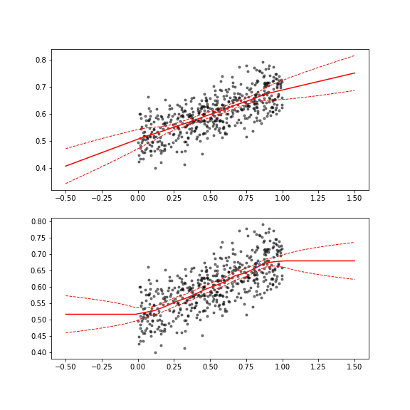
In many cases, one needs to approximate a function from noisy measurements. To get the smooth underlying trend behind the data, one often uses techniques like LOESS. An alternative way is to discretize the function onto a grid and treat the function values at the grid points as unknowns. In order to get smooth trends, one can add a prior (penalization term) that favors smoothness. In the helper function `smooth_interp1`, one can specify priors for the first and second order differences between the function values. The choice of using first or second order smoothness priors affects the extrapolation behavior of the function, as demonstrated below.
```python
import numpy as np
import blinpy as bp
import matplotlib.pyplot as plt
# generate data
xobs = np.random.random(500)
ysig = 0.05
yobs = 0.5+0.2*xobs + ysig*np.random.randn(len(xobs))
# define grid for fitting
xfit = np.linspace(-0.5,1.5,30)
# fit with second order difference prior
yfit1, yfit_icov1 = bp.models.smooth_interp1(xfit, xobs, yobs, obs_cov=ysig**2, d2_var=1e-5)
yfit_cov1 = np.linalg.inv(yfit_icov1)
# fit with first order difference prior
yfit2, yfit_icov2 = bp.models.smooth_interp1(xfit, xobs, yobs, obs_cov=ysig**2, d1_var=1e-4)
yfit_cov2 = np.linalg.inv(yfit_icov2)
# plot results
plt.figure(figsize=(8,8))
plt.subplot(211)
plt.plot(xobs,yobs,'k.', alpha=0.5)
plt.plot(xfit, yfit1, 'r-')
plt.plot(xfit, yfit1+2*np.sqrt(np.diag(yfit_cov1)), 'r--', lw=1)
plt.plot(xfit, yfit1-2*np.sqrt(np.diag(yfit_cov1)), 'r--', lw=1)
plt.subplot(212)
plt.plot(xobs,yobs,'k.', alpha=0.5)
plt.plot(xfit, yfit2, 'r-')
plt.plot(xfit, yfit2+2*np.sqrt(np.diag(yfit_cov2)), 'r--', lw=1)
plt.plot(xfit, yfit2-2*np.sqrt(np.diag(yfit_cov2)), 'r--', lw=1)
plt.show()
```
### Generalized Additive Models (GAM): line fit
The `GamModel` class offers a more general interface to linear model fitting. With `GamModel` one can fit models that consist of components that represent `N` columns in the final system matrix. Priors can be given (optional) for each block. For instance, the line fitting example, where a prior is given for the slope, is solved with `GamModel` as follows:
```python
import numpy as np
import pandas as pd
from blinpy.models import GamModel
data = pd.DataFrame(
{'x': np.array([0.0, 1.0, 1.0, 2.0, 1.8, 3.0, 4.0, 5.2, 6.5, 8.0, 10.0]),
'y': np.array([5.0, 5.0, 5.1, 5.3, 5.5, 5.7, 6.0, 6.3, 6.7, 7.1, 7.5])}
)
gam_specs = [
{
'fun': lambda df: df['x'].values[:, np.newaxis],
'name': 'slope',
'prior': {
'B': np.eye(1),
'mu': np.array([0.35]),
'cov': np.array([0.001])
}
},
{
'fun': lambda df: np.ones((len(df), 1)),
'name': 'bias'
}
]
model = GamModel('y', gam_specs).fit(data)
model.theta
{'slope': array([0.34251082]), 'bias': array([4.60393546])}
```
That is, one feeds in a list of dicts that specify the GAM components. Each dict must contain a function that returns the system matrix columns and a name for the model component. Optionally, one can specify a Gaussian prior for the components. The `GamModel` class then compiles and fits the linear-Gaussian system.
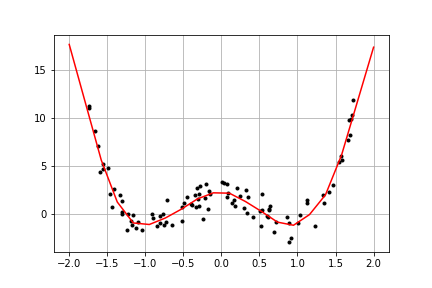
### GAM: non-parametric regression
Let us take a slightly more non-trivial example of a GAM, where we model an unknown function in a grid of selected input points. Points in between are linearly interpolated. Moreover, we impose a second order difference prior on the function values to enforce smoothness. The interpolation matrix and difference prior construction are done with utility functions provided in the package. The example code is given below:
```python
import numpy as np
import pandas as pd
import blinpy as bp
import matplotlib.pyplot as plt
xobs = -1.75 + 3.5*np.random.random(100)
yobs = 3*xobs**4-6*xobs**2+2 + np.random.randn(len(xobs))
data = pd.DataFrame({'x': xobs, 'y': yobs})
xfit = np.linspace(-2,2,20)
nfit = len(xfit)
gam_spec = [
{
'fun': lambda df: bp.utils.interp_matrix(df['x'].values, xfit),
'name': 'smoothfun',
'prior': {
'B': bp.utils.diffmat(nfit, order=2),
'mu': np.zeros(nfit-2),
'cov': np.ones(nfit-2)
}
}
]
model = bp.models.GamModel('y', gam_spec).fit(data)
print(model.theta)
plt.figure(figsize=(6,4))
plt.plot(xobs, yobs, 'k.')
plt.plot(xfit, model.post_mu, 'r-')
plt.grid(True)
plt.show()
{'smoothfun': array([16.83584518, 11.41451668, 5.99318818, 1.70894339, -0.57917346,
-1.10535146, -0.62246082, 0.95388427, 1.88575506, 2.07577794,
2.19637689, 1.61404071, 0.48381775, -0.22563978, -0.74711054,
-0.82681361, 0.84100582, 4.54902101, 8.76411573, 12.97921046])}
```
GAM models give a nice way to blend parametric and nonparametric regression models together.
Raw data
{
"_id": null,
"home_page": "https://github.com/solbes/blinpy",
"name": "blinpy",
"maintainer": null,
"docs_url": null,
"requires_python": null,
"maintainer_email": null,
"keywords": "bayes, linear, gam",
"author": "Antti Solonen",
"author_email": "antti.solonen@gmail.com",
"download_url": "https://files.pythonhosted.org/packages/04/5c/3b04780c4ad515251dec1b4c97b3ed1de815fcf331d3e0441622c6f51ced/blinpy-0.1.12.tar.gz",
"platform": null,
"description": "# blinpy - Bayesian LINear models in PYthon\n\nWhen applying linear regression models in practice, one often ends up going \nback to the basic formulas to figure out how things work, especially if \nGaussian priors are applied. This package is built for this (almost trivial) \ntask of fitting linear-Gaussian models. The package includes a basic numpy \nengine for fitting a general linear-Gaussian model, plus some model classes \nthat provide a simple interface for working with the models.\n\nIn the end, before fitting a specified model, the model is always transformed\ninto the following form:\n\nLikelihood: y = Aθ + N(0, Γ<sub>obs</sub>)\n\nPrior: Bθ ~ N(μ<sub>pr</sub>, Γ<sub>obs</sub>).\n\nIf one has the system already in suitable numpy arrays, one can directly use \nthe numpy engine to fit the above system. However, some model classes are \ndefined as well that make it easy to define and work with some common types \nof linear-Gaussian models, see the examples below.\n\n## Installation\n\n`pip install blinpy`\n\n## Examples\n\n### Fitting a line, no priors\n\nStandard linear regression can be easily done with \n`blinpy.models.LinearModel` class that takes in the input data as a `pandas` \nDataFrame.\n\nLet us fit a model y=θ<sub>0</sub> + θ<sub>1</sub>x + e using \nsome dummy data:\n\n```python\nimport pandas as pd\nimport numpy as np\nfrom blinpy.models import LinearModel\n\ndata = pd.DataFrame(\n {'x': np.array([0.0, 1.0, 1.0, 2.0, 1.8, 3.0, 4.0, 5.2, 6.5, 8.0, 10.0]),\n 'y': np.array([5.0, 5.0, 5.1, 5.3, 5.5, 5.7, 6.0, 6.3, 6.7, 7.1, 7.5])}\n)\n\nlm = LinearModel(\n output_col='y', \n input_cols=['x'],\n bias = True,\n theta_names=['th1'],\n).fit(data)\n\nprint(lm.theta)\n```\n\nThat is, the model is defined in the constructor, and fitted using the `fit` \nmethod. The fitted parameters can be accessed via `lm.theta` property. The \ncode outputs:\n```python\n{'bias': 4.8839773707086165, 'th1': 0.2700293864048287}\n```\n\nThe posterior mean and covariance information are also stored in numpy arrays\nas `lm.post_mu` and `lm.post_icov`. Note that the posterior precision matrix\n(inverse of covariance) is given instead of the covariance matrix.\n\n### Fit a line with priors\n\nGaussian priors (mean and cov) can be added to the `fit` method of `LinearModel`. Let us take the same example as above, but now add a prior `bias ~ N(4,1)` and `th1 ~ N(0.35, 0.001)`:\n\n```python\nlm = LinearModel(\n output_col='y', \n input_cols=['x'],\n bias = True,\n theta_names=['th1'],\n).fit(data, pri_mu=[4.0, 0.35], pri_cov=[1.0, 0.001])\n\nprint(lm.theta)\n\n{'bias': 4.546825637808106, 'th1': 0.34442570226594676}\n```\n\nThe prior covariance can be given as a scalar, vector or matrix. If it's a scalar, the same variance is applied for all parameters. If it's a vector, like in the example above, the variances for individual parameters are given by the vector elements. A full matrix can be used if the parameters correlate a priori.\n\n### Fit a line with partial priors\n\nSometimes we don't want to put priors for all the parameters, but just for a subset of them. `LinearModel` supports this via the `pri_cols` argument in the model constructor. For instance, let us now fit the same model as above, but only put the prior `th1 ~ N(0.35, 0.001)` and no prior for the bias term:\n\n```python\nlm = LinearModel(\n output_col='y', \n input_cols=['x'],\n bias = True,\n theta_names=['th1'],\n pri_cols = ['th1']\n).fit(data, pri_mu=[0.35], pri_cov=[0.001])\n\nprint(lm.theta)\n\n{'bias': 4.603935457929664, 'th1': 0.34251082265349875}\n```\n\n### Using the numpy engine directly\n\nFor some more complex linear models, one might want to use the numpy linear fitting function directly. The function is found from `blinpy.utils.linfit`, an example of how to fit the above example is given below:\n\n```python\nimport numpy as np\nfrom blinpy.utils import linfit\n\nx = np.array([0.0, 1.0, 1.0, 2.0, 1.8, 3.0, 4.0, 5.2, 6.5, 8.0, 10.0])\ny = np.array([5.0, 5.0, 5.1, 5.3, 5.5, 5.7, 6.0, 6.3, 6.7, 7.1, 7.5])\n\nX = np.concatenate((np.ones((11, 1)), x[:, np.newaxis]), axis=1)\n\nmu, icov, _ = linfit(y, X, pri_mu=[4.0, 0.35], pri_cov=[1.0, 0.001])\nprint(mu)\n\n[4.54682564 0.3444257]\n```\nOne can give the optional prior transformation matrix `B` as an input to the `linfit` function, by default `B` is identity.\n\n### Smoothed interpolation \n\nIn many cases, one needs to approximate a function from noisy measurements. To get the smooth underlying trend behind the data, one often uses techniques like LOESS. An alternative way is to discretize the function onto a grid and treat the function values at the grid points as unknowns. In order to get smooth trends, one can add a prior (penalization term) that favors smoothness. In the helper function `smooth_interp1`, one can specify priors for the first and second order differences between the function values. The choice of using first or second order smoothness priors affects the extrapolation behavior of the function, as demonstrated below.\n\n```python\nimport numpy as np\nimport blinpy as bp\nimport matplotlib.pyplot as plt\n\n# generate data\nxobs = np.random.random(500)\nysig = 0.05\nyobs = 0.5+0.2*xobs + ysig*np.random.randn(len(xobs))\n\n# define grid for fitting\nxfit = np.linspace(-0.5,1.5,30)\n\n# fit with second order difference prior\nyfit1, yfit_icov1 = bp.models.smooth_interp1(xfit, xobs, yobs, obs_cov=ysig**2, d2_var=1e-5)\nyfit_cov1 = np.linalg.inv(yfit_icov1)\n\n# fit with first order difference prior\nyfit2, yfit_icov2 = bp.models.smooth_interp1(xfit, xobs, yobs, obs_cov=ysig**2, d1_var=1e-4)\nyfit_cov2 = np.linalg.inv(yfit_icov2)\n\n# plot results\nplt.figure(figsize=(8,8))\nplt.subplot(211)\nplt.plot(xobs,yobs,'k.', alpha=0.5)\nplt.plot(xfit, yfit1, 'r-')\nplt.plot(xfit, yfit1+2*np.sqrt(np.diag(yfit_cov1)), 'r--', lw=1)\nplt.plot(xfit, yfit1-2*np.sqrt(np.diag(yfit_cov1)), 'r--', lw=1)\n\nplt.subplot(212)\nplt.plot(xobs,yobs,'k.', alpha=0.5)\nplt.plot(xfit, yfit2, 'r-')\nplt.plot(xfit, yfit2+2*np.sqrt(np.diag(yfit_cov2)), 'r--', lw=1)\nplt.plot(xfit, yfit2-2*np.sqrt(np.diag(yfit_cov2)), 'r--', lw=1)\n\nplt.show()\n```\n\n\n\n### Generalized Additive Models (GAM): line fit\n\nThe `GamModel` class offers a more general interface to linear model fitting. With `GamModel` one can fit models that consist of components that represent `N` columns in the final system matrix. Priors can be given (optional) for each block. For instance, the line fitting example, where a prior is given for the slope, is solved with `GamModel` as follows:\n\n```python\nimport numpy as np\nimport pandas as pd\nfrom blinpy.models import GamModel\n\ndata = pd.DataFrame(\n {'x': np.array([0.0, 1.0, 1.0, 2.0, 1.8, 3.0, 4.0, 5.2, 6.5, 8.0, 10.0]),\n 'y': np.array([5.0, 5.0, 5.1, 5.3, 5.5, 5.7, 6.0, 6.3, 6.7, 7.1, 7.5])}\n)\n\ngam_specs = [\n {\n 'fun': lambda df: df['x'].values[:, np.newaxis],\n 'name': 'slope',\n 'prior': {\n 'B': np.eye(1),\n 'mu': np.array([0.35]),\n 'cov': np.array([0.001])\n }\n },\n {\n 'fun': lambda df: np.ones((len(df), 1)),\n 'name': 'bias'\n }\n]\n\nmodel = GamModel('y', gam_specs).fit(data)\nmodel.theta\n\n{'slope': array([0.34251082]), 'bias': array([4.60393546])}\n```\n\nThat is, one feeds in a list of dicts that specify the GAM components. Each dict must contain a function that returns the system matrix columns and a name for the model component. Optionally, one can specify a Gaussian prior for the components. The `GamModel` class then compiles and fits the linear-Gaussian system.\n\n### GAM: non-parametric regression\n\nLet us take a slightly more non-trivial example of a GAM, where we model an unknown function in a grid of selected input points. Points in between are linearly interpolated. Moreover, we impose a second order difference prior on the function values to enforce smoothness. The interpolation matrix and difference prior construction are done with utility functions provided in the package. The example code is given below:\n\n```python\nimport numpy as np\nimport pandas as pd\nimport blinpy as bp\nimport matplotlib.pyplot as plt\n\nxobs = -1.75 + 3.5*np.random.random(100)\nyobs = 3*xobs**4-6*xobs**2+2 + np.random.randn(len(xobs))\ndata = pd.DataFrame({'x': xobs, 'y': yobs})\n\nxfit = np.linspace(-2,2,20)\nnfit = len(xfit)\n\ngam_spec = [\n {\n 'fun': lambda df: bp.utils.interp_matrix(df['x'].values, xfit),\n 'name': 'smoothfun',\n 'prior': {\n 'B': bp.utils.diffmat(nfit, order=2),\n 'mu': np.zeros(nfit-2),\n 'cov': np.ones(nfit-2)\n }\n }\n]\n\nmodel = bp.models.GamModel('y', gam_spec).fit(data)\nprint(model.theta)\n\nplt.figure(figsize=(6,4))\nplt.plot(xobs, yobs, 'k.')\nplt.plot(xfit, model.post_mu, 'r-')\nplt.grid(True)\nplt.show()\n\n{'smoothfun': array([16.83584518, 11.41451668, 5.99318818, 1.70894339, -0.57917346,\n -1.10535146, -0.62246082, 0.95388427, 1.88575506, 2.07577794,\n 2.19637689, 1.61404071, 0.48381775, -0.22563978, -0.74711054,\n -0.82681361, 0.84100582, 4.54902101, 8.76411573, 12.97921046])}\n```\n\n\nGAM models give a nice way to blend parametric and nonparametric regression models together.\n",
"bugtrack_url": null,
"license": "MIT",
"summary": "Bayesian Linear Models in Python",
"version": "0.1.12",
"project_urls": {
"Download": "https://github.com/solbes/blinpy/archive/refs/tags/0.1.12.tar.gz",
"Homepage": "https://github.com/solbes/blinpy"
},
"split_keywords": [
"bayes",
" linear",
" gam"
],
"urls": [
{
"comment_text": "",
"digests": {
"blake2b_256": "045c3b04780c4ad515251dec1b4c97b3ed1de815fcf331d3e0441622c6f51ced",
"md5": "8bb0da2c108ce5d4ea6a60ca87cf65c7",
"sha256": "32c327322730479738913a5951862f60ed5bf9be2fcf0fc130d52bc2b66ff6f5"
},
"downloads": -1,
"filename": "blinpy-0.1.12.tar.gz",
"has_sig": false,
"md5_digest": "8bb0da2c108ce5d4ea6a60ca87cf65c7",
"packagetype": "sdist",
"python_version": "source",
"requires_python": null,
"size": 18112,
"upload_time": "2024-09-27T08:17:19",
"upload_time_iso_8601": "2024-09-27T08:17:19.827458Z",
"url": "https://files.pythonhosted.org/packages/04/5c/3b04780c4ad515251dec1b4c97b3ed1de815fcf331d3e0441622c6f51ced/blinpy-0.1.12.tar.gz",
"yanked": false,
"yanked_reason": null
}
],
"upload_time": "2024-09-27 08:17:19",
"github": true,
"gitlab": false,
"bitbucket": false,
"codeberg": false,
"github_user": "solbes",
"github_project": "blinpy",
"travis_ci": false,
"coveralls": false,
"github_actions": false,
"lcname": "blinpy"
}

