


Table of contents
=================
* [BSXplorer](#bsxplorer)
* [How to cite](#how-to-cite)
* [Installation](#installation)
* [Usage](#usage)
* [API usage](#api-usage)
* [Basic usage](#basic-usage)
* [Methylation pattern clusterisation](#clusterisation)
* [Chromosome methylation levels](#chromosome-methylation-levels)
* [Gene body methylation](#gene-body-methylation)
* [Different organisms analysis](#different-organisms-analysis)
* [Enrichment of DMRs](#enrichment-of-dmrs)
* [Other functionality](#other-functionality)
* [Console usage](#console-usage)
* [What's new](#whats-new)
BSXplorer
=========
Analytical framework for BS-seq data comparison and visualization.
BSXplorer facilitates efficient methylation data mining,
contrasting and visualization, making it an easy-to-use package
that is highly useful for epigenetic research.
For Python API reference manual and tutorials visit: https://shitohana.github.io/BSXplorer.

<details>
<summary>How to cite</summary>
## How to cite
If you use our package in your research, please consider
citing our paper.
Yuditskiy, K., Bezdvornykh, I., Kazantseva, A. et al. BSXplorer:
analytical framework for exploratory analysis of BS-seq data. BMC
Bioinformatics 25, 96 (2024). https://doi.org/10.1186/s12859-024-05722-9
</details>
Installation
------------
To install latest stable version:
```commandline
pip install bsxplorer
```
If you want to install the prerelease version (dev branch):
```commandline
pip install pip install git+https://github.com/shitohana/BSXplorer.git@dev
```
Usage
-----

In this project our aim was to create a both powerful and flexible tool
to facilitate exploratory data analysis of BS-Seq data obtained in non-model
organisms (BSXplorer works for model organisms as well). That's why BSXplorer
is implemented as a Python package. Modular structure of BSXplorer together
with easy to use and configurable API makes it a highly integratable and
scalable package for a wide range of applications in bioinformatical projects.
Even though BSXplorer is available as console application, to fully utilize
its potential _consider using it as a python package_. [Detailed documentation
can be found here](https://shitohana.github.io/BSXplorer).
API usage
---------
```python
import bsxplorer as bsx
```
### Basic usage
The main objects in BSXplorer are the `Genome` and `Metagene`, `MetageneFiles`
classes. `Genome` class is used for reading and filtering genomic annotation data.
```python
genome = bsx.Genome.from_gff("path/to/annotation.gff")
```
Even though here `genome` was created with `.from_gff` constructor, to read custom
annotation format (TSV file), use `.from_custom` and specify column indexes (0-based).
Once we have read annotation file, methylation report can be processed via `Metagene`
class (or `MetageneFiles` for multiple reports).
```python
metagene = bsx.Metagene.from_bismark(
"path/to/report.txt",
genome=genome.gene_body(min_length=0, flank_length=2000),
up_windows=100, body_windows=200, down_windows=100
)
```
Here we have read methylation report file. Methylation data has been read only
for gene bodies (`genome.gene_body(min_length=0, flank_length=2000)`) with
200 windows resolution for gene body (`body_windows=200`) and 100 for flanking
regions (`up_windows=100, down_windows=100`).
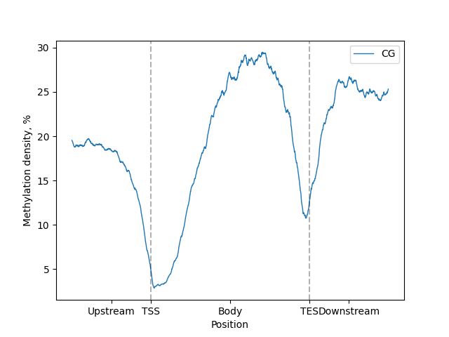
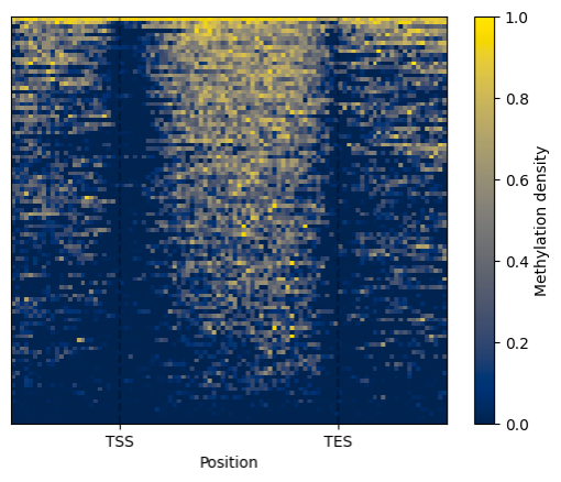
Now we can generate visualiztions.
```python
filtered = metagene.filter(context="CG")
filtered.line_plot().draw_mpl()
filtered.heat_map().draw_mpl()
```
BSXplorer can generate plots with two plotting libraries: matplotlib and Plotly.
`_mpl` in methods names stands for matplotlib and `_plotly` for Plotly.
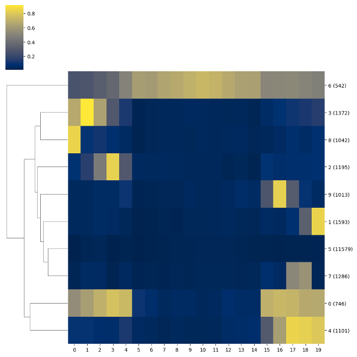
### Clusterisation
BSXplorer allows for discovery of gene modules characterised with similar methylation patterns.
Once the data was filtered based on methylation context and strand,
one can use the `.cluster()` method. The resulting object contains an
ordered list of clustered genes and their visualisation in a form of a heatmap.
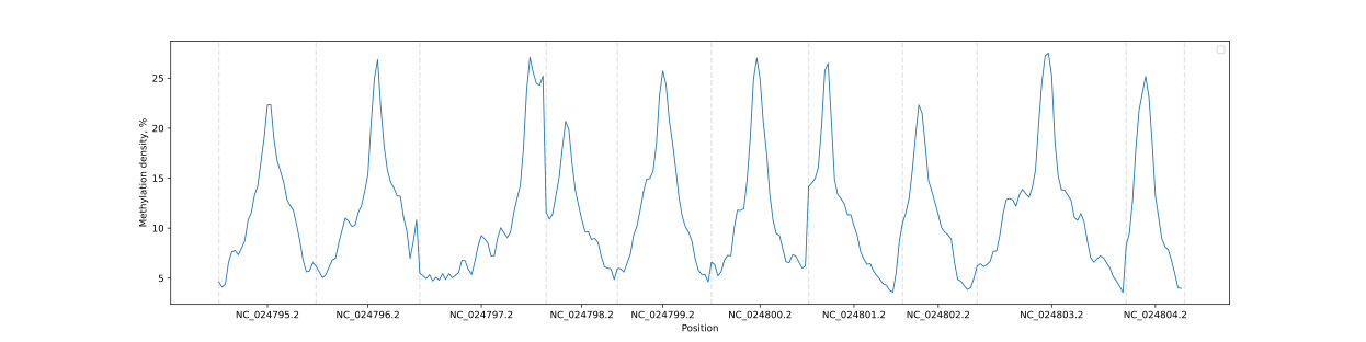
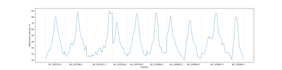
### Chromosome methylation levels
BSXplorer allows a user to visualize the overall methylation levels of
chromosomes using the corresponding ChrLevels object:
```python
levels = bsx.ChrLevels.from_bismark("path/to/report.txt", chr_min_length=10**6, window_length=10**6)
levels.draw_mpl(smooth=5)
```
In a way that is similar to the Metagene method, the methylation data
can be subjected to filtering to selectively display a methylation
context that is of interest.
```python
levels.filter(context="CG").draw_mpl(smooth=5)
```
### Gene body methylation
BSXplorer allows for the categorization of regions based on their methylation level and density.
This is done by assuming that cytosine methylation levels follow a binomial distribution,
as explained in Takuno and Gaut's research (please refer to
**[1, 2]** https://doi.org/10.1073/pnas.1215380110 for details).
The genes are then divided into three categories,
BM (body-methylated), IM (intermediately-methylated) and UM (under-methylated),
based on their methylation levels in the CG context using the following formula.
$$ CG<P_{CG};\ \ CHG/CHH>1-P_{CG} $$
$$ P_{CG}\le CG<1-P_{CG};\ \ CHG/CHH>1-P_{CG} $$
$$ CG/CHG/CHH>1-P_{CG} $$
The same rationale may be applied to other methylation contexts,
as BSXplorer can produce $P_{CHG}$ and $P_{CHH}$ for CHG sites and CHH sites, respectively.
**[1]** _Takuno S, Gaut BS. Body-Methylated Genes in Arabidopsis thaliana
Are Functionally Important and Evolve Slowly. Mol Biol Evol. 2012;29:219–27._
**[2]** _Takuno S, Gaut BS. Gene body methylation is conserved between
plant orthologs and is of evolutionary consequence. Proc Natl Acad Sci. 2013;110:1797–802._
```python
# Calculate pvalue for cytosine methylation via binomial test
binom_data = bsx.BinomialData.from_report(
"path/to/report.txt",
report_type="bismark"
)
# Created binomial data object can now be used to calculate pvalues
# for methylation of genomic regions
region_stats = binom_data.region_pvalue(genome.gene_body(), methylation_pvalue=.01)
# .categorise method returns tuple of three DataFrames
# for BM, IM and UM genes respectively
bm, im, um = region_stats.categorise(context="CG", p_value=.05)
# Now we can create MetageneFiles object to visualize methylation pattern
# of categorised groups
cat_metagene = bsx.MetageneFiles([
metagene.filter(context="CG", genome=bm),
metagene.filter(context="CG", genome=im),
metagene.filter(context="CG", genome=um),
], labels=["BM", "IM", "UM"])
# And plot it
tick_labels = ["-2000kb", "TSS", "", "TES", "+2000kb"]
cat_metagene.line_plot().draw_mpl(tick_labels=tick_labels)
```

### Different organisms analysis
Start with import of genome annotation data for species of interest.
```python
arath_genes = bsxplorer.Genome.from_gff("arath_genome.gff").gene_body(min_length=0)
bradi_genes = bsxplorer.Genome.from_gff("bradi_genome.gff").gene_body(min_length=0)
mouse_genes = bsxplorer.Genome.from_gff("musmu_genome.gff").gene_body(min_length=0)
```
Next, read in cytosine reports for each sample separately:
```python
window_kwargs = dict(up_windows=200, body_windows=400, down_windows=200)
arath_metagene = bsx.Metagene.from_bismark("arath_example.txt", arath_genes, **window_kwargs)
bradi_metagene = bsx.Metagene.from_bismark("bradi_example.txt", bradi_genes, **window_kwargs)
musmu_metagene = bsx.Metagene.from_bismark("musmu_example.txt", mouse_genes, **window_kwargs)
```
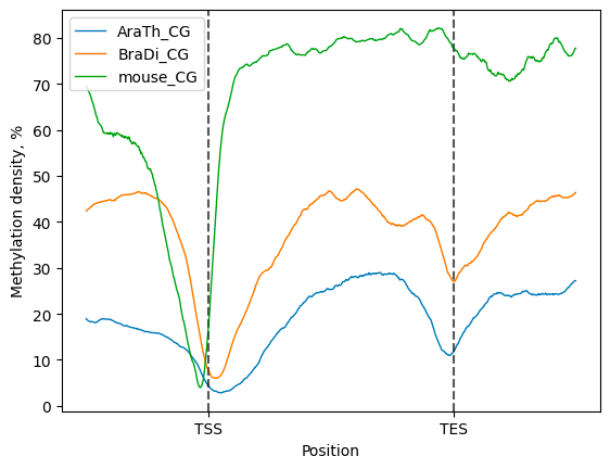
To perform comparative analysis, initialize the `bsxplorer.MetageneFiles`
class using metagene data in a vector format, where labels for every organism
are provided explicitly.
Next, apply methylation context and strand filters to the input files:
```python
filtered = files.filter("CG", "+")
```
Then, a compendium of line plots to guide a comparative analyses of methylation patterns in
different species is constructed:
```python
filtered.line_plot(smooth=50).draw_mpl()
```
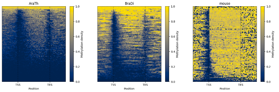
The line plot representation may be further supplemented by a heatmap:
```python
filtered.heat_map(100, 100).draw_mpl()
```
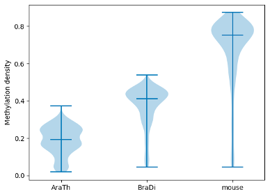
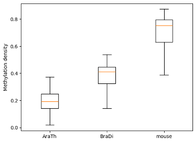
To examine and highlight differences in methylation patterns between
different organisms, summary statistics is made available in a graphical format.
```python
filtered.box_plot(violin=True).draw_mpl()
filtered.box_plot().draw_mpl()
```
### Enrichment of DMRs
BSXplorer offers functionality to align one set of regions over another. Regions can
be read either with :class:`Genome` or initialized directly with
`polars functionality <https://docs.pola.rs/api/python/stable/reference/api/polars.read_csv.html>`_
(DataFrame need to have `chr`, `start` and `end` columns).
To align regions (e.g. define DMR position relative to genes) or perform the enrichment of regions at these
genomic features against the genome background use :class:`Enrichment`.
```python
# If you want to perform an ENRICHMENT, and not only plot
# the density of metagene coverage, you NEED to use .raw() method
# for genome DataFrame.
genes = bsx.Genome.from_gff("path/to/annot.gff").raw()
dmr = bsx.Genome.from_custom(
"path/to/dmr.txt",
chr_col=0, # Theese columns indexes are configurable
start_col=1,
end_col=2
).all()
enrichment = bsx.Enrichment(dmr, genes, flank_length=2000).enrich()
```

`Enrichment.enrich` returns `EnrichmentResult`, which stores enrichment
statistics and coordinates of regions which have aligned with
genomic features. The metagene coverage with regions
can be plotted via `EnrichmentResult.plot_density_mpl` method.
```python
fig = enrichment.plot_density_mpl(
tick_labels=["-2000bp", "TSS", "Gene body", "TES" "+2000bp"],
)
```

Enrichment statistics can be accessed with `EnrichmentResult.enrich_stats`
or plotted with `EnrichmentResult.plot_enrich_mpl`
```python
enrichment.plot_enrich_mpl()
```

### Other functionality
For other functionality, such as methylation reports conversion and BAM conversion and
statistics please refer to the [documentation](https://shitohana.github.io/BSXplorer).
Console usage
-------------
BSXplorer can be used in a console mode for generating complex HTML-reports
([see example here](https://shitohana.github.io/BSXplorer/_static/html/metagene_intra.html)) and
running many analysis at once or converting BAM to methylation report. For detailed
commands description and examples, please refer to
the [documentation](https://shitohana.github.io/BSXplorer/_console.html).
What's new
-------------------------------------------------
Since publication we have released Version `1.1.0`.
### Major changes
* Added new classes for Unified reading of
methylation reports (`UniversalReader`, `UniversalReplicatesReader`).
Now any supported report type can be converted into another.
* Added support for processing BAM files (`BAMReader`).
BAM files can be either converted to methylation report
(faster than with native methods), or methylation statistics,
such as methylation entropy, epipolymorphism or PDR can
be calculated.
* Added method for aligning one set of regions along another
(e.g. DMR along genes) – `Enrichment`. Regions can not only be
aligned, but the coverage of the metagene by DMRs can
be visualized.
### Other improvements
* Any plot data now can be retrieved by corresponding method.
* Fixes to the plotting API.
* Fixes to `Category` report.
* Added console command for processing BAM files.
Raw data
{
"_id": null,
"home_page": null,
"name": "bsxplorer",
"maintainer": null,
"docs_url": null,
"requires_python": ">=3.10",
"maintainer_email": null,
"keywords": "bismark, bs-seq, methylation, plot",
"author": null,
"author_email": "Konstantin Y <kyudytskiy@gmail.com>",
"download_url": "https://files.pythonhosted.org/packages/60/93/8ec982135ff4d0dcb46f06474c117b4b6127b1663037f7f87a463908801c/bsxplorer-1.1.0.post2.tar.gz",
"platform": null,
"description": "\n\n\n \n\n\nTable of contents\n=================\n\n* [BSXplorer](#bsxplorer)\n * [How to cite](#how-to-cite)\n * [Installation](#installation)\n * [Usage](#usage)\n * [API usage](#api-usage)\n * [Basic usage](#basic-usage)\n * [Methylation pattern clusterisation](#clusterisation)\n * [Chromosome methylation levels](#chromosome-methylation-levels)\n * [Gene body methylation](#gene-body-methylation)\n * [Different organisms analysis](#different-organisms-analysis)\n * [Enrichment of DMRs](#enrichment-of-dmrs)\n * [Other functionality](#other-functionality)\n * [Console usage](#console-usage)\n * [What's new](#whats-new)\n \n\nBSXplorer\n=========\n\nAnalytical framework for BS-seq data comparison and visualization. \nBSXplorer facilitates efficient methylation data mining, \ncontrasting and visualization, making it an easy-to-use package \nthat is highly useful for epigenetic research.\n\nFor Python API reference manual and tutorials visit: https://shitohana.github.io/BSXplorer.\n\n\n\n<details>\n<summary>How to cite</summary>\n\n## How to cite\n\nIf you use our package in your research, please consider\nciting our paper.\n\nYuditskiy, K., Bezdvornykh, I., Kazantseva, A. et al. BSXplorer: \nanalytical framework for exploratory analysis of BS-seq data. BMC \nBioinformatics 25, 96 (2024). https://doi.org/10.1186/s12859-024-05722-9\n\n</details>\n\nInstallation\n------------\n\nTo install latest stable version:\n\n```commandline\npip install bsxplorer\n```\n\nIf you want to install the prerelease version (dev branch):\n\n```commandline\npip install pip install git+https://github.com/shitohana/BSXplorer.git@dev\n```\n\nUsage\n-----\n\n\n\nIn this project our aim was to create a both powerful and flexible tool\nto facilitate exploratory data analysis of BS-Seq data obtained in non-model\norganisms (BSXplorer works for model organisms as well). That's why BSXplorer\nis implemented as a Python package. Modular structure of BSXplorer together\nwith easy to use and configurable API makes it a highly integratable and\nscalable package for a wide range of applications in bioinformatical projects.\n\nEven though BSXplorer is available as console application, to fully utilize\nits potential _consider using it as a python package_. [Detailed documentation\ncan be found here](https://shitohana.github.io/BSXplorer).\n \n\nAPI usage\n---------\n\n```python\nimport bsxplorer as bsx\n```\n\n### Basic usage\n\nThe main objects in BSXplorer are the `Genome` and `Metagene`, `MetageneFiles`\nclasses. `Genome` class is used for reading and filtering genomic annotation data.\n\n```python\ngenome = bsx.Genome.from_gff(\"path/to/annotation.gff\")\n```\n\nEven though here `genome` was created with `.from_gff` constructor, to read custom\nannotation format (TSV file), use `.from_custom` and specify column indexes (0-based).\n\nOnce we have read annotation file, methylation report can be processed via `Metagene`\nclass (or `MetageneFiles` for multiple reports).\n\n```python\nmetagene = bsx.Metagene.from_bismark(\n \"path/to/report.txt\",\n genome=genome.gene_body(min_length=0, flank_length=2000),\n up_windows=100, body_windows=200, down_windows=100\n)\n```\n\nHere we have read methylation report file. Methylation data has been read only\nfor gene bodies (`genome.gene_body(min_length=0, flank_length=2000)`) with \n200 windows resolution for gene body (`body_windows=200`) and 100 for flanking\nregions (`up_windows=100, down_windows=100`).\n\nNow we can generate visualiztions.\n\n```python\nfiltered = metagene.filter(context=\"CG\")\nfiltered.line_plot().draw_mpl()\nfiltered.heat_map().draw_mpl()\n```\n\n\n\n\n\nBSXplorer can generate plots with two plotting libraries: matplotlib and Plotly.\n`_mpl` in methods names stands for matplotlib and `_plotly` for Plotly.\n\n### Clusterisation\n\nBSXplorer allows for discovery of gene modules characterised with similar methylation patterns.\n\nOnce the data was filtered based on methylation context and strand, \none can use the `.cluster()` method. The resulting object contains an \nordered list of clustered genes and their visualisation in a form of a heatmap.\n\n\n\n### Chromosome methylation levels\n\nBSXplorer allows a user to visualize the overall methylation levels of \nchromosomes using the corresponding ChrLevels object:\n\n```python\nlevels = bsx.ChrLevels.from_bismark(\"path/to/report.txt\", chr_min_length=10**6, window_length=10**6)\nlevels.draw_mpl(smooth=5)\n```\n\n\n\nIn a way that is similar to the Metagene method, the methylation data \ncan be subjected to filtering to selectively display a methylation \ncontext that is of interest.\n\n```python\nlevels.filter(context=\"CG\").draw_mpl(smooth=5)\n```\n\n\n\n### Gene body methylation\n\nBSXplorer allows for the categorization of regions based on their methylation level and density. \nThis is done by assuming that cytosine methylation levels follow a binomial distribution, \nas explained in Takuno and Gaut's research (please refer to \n**[1, 2]** https://doi.org/10.1073/pnas.1215380110 for details). \nThe genes are then divided into three categories, \nBM (body-methylated), IM (intermediately-methylated) and UM (under-methylated), \nbased on their methylation levels in the CG context using the following formula.\n\n$$ CG<P_{CG};\\ \\ CHG/CHH>1-P_{CG} $$\n\n$$ P_{CG}\\le CG<1-P_{CG};\\ \\ CHG/CHH>1-P_{CG} $$\n\n$$ CG/CHG/CHH>1-P_{CG} $$\n\nThe same rationale may be applied to other methylation contexts, \nas BSXplorer can produce $P_{CHG}$ and $P_{CHH}$ for CHG sites and CHH sites, respectively. \n\n**[1]** _Takuno S, Gaut BS. Body-Methylated Genes in Arabidopsis thaliana \nAre Functionally Important and Evolve Slowly. Mol Biol Evol. 2012;29:219\u201327._\n\n**[2]** _Takuno S, Gaut BS. Gene body methylation is conserved between \nplant orthologs and is of evolutionary consequence. Proc Natl Acad Sci. 2013;110:1797\u2013802._\n\n```python\n# Calculate pvalue for cytosine methylation via binomial test\nbinom_data = bsx.BinomialData.from_report(\n \"path/to/report.txt\",\n report_type=\"bismark\"\n)\n\n# Created binomial data object can now be used to calculate pvalues\n# for methylation of genomic regions\nregion_stats = binom_data.region_pvalue(genome.gene_body(), methylation_pvalue=.01)\n# .categorise method returns tuple of three DataFrames\n# for BM, IM and UM genes respectively\nbm, im, um = region_stats.categorise(context=\"CG\", p_value=.05)\n\n# Now we can create MetageneFiles object to visualize methylation pattern\n# of categorised groups\ncat_metagene = bsx.MetageneFiles([\n metagene.filter(context=\"CG\", genome=bm),\n metagene.filter(context=\"CG\", genome=im),\n metagene.filter(context=\"CG\", genome=um),\n], labels=[\"BM\", \"IM\", \"UM\"])\n\n# And plot it\ntick_labels = [\"-2000kb\", \"TSS\", \"\", \"TES\", \"+2000kb\"]\ncat_metagene.line_plot().draw_mpl(tick_labels=tick_labels)\n```\n\n\n\n### Different organisms analysis\n\nStart with import of genome annotation data for species of interest.\n\n```python\narath_genes = bsxplorer.Genome.from_gff(\"arath_genome.gff\").gene_body(min_length=0)\nbradi_genes = bsxplorer.Genome.from_gff(\"bradi_genome.gff\").gene_body(min_length=0)\nmouse_genes = bsxplorer.Genome.from_gff(\"musmu_genome.gff\").gene_body(min_length=0)\n```\n\nNext, read in cytosine reports for each sample separately:\n\n```python\nwindow_kwargs = dict(up_windows=200, body_windows=400, down_windows=200)\n\narath_metagene = bsx.Metagene.from_bismark(\"arath_example.txt\", arath_genes, **window_kwargs)\nbradi_metagene = bsx.Metagene.from_bismark(\"bradi_example.txt\", bradi_genes, **window_kwargs)\nmusmu_metagene = bsx.Metagene.from_bismark(\"musmu_example.txt\", mouse_genes, **window_kwargs)\n```\n\nTo perform comparative analysis, initialize the `bsxplorer.MetageneFiles` \nclass using metagene data in a vector format, where labels for every organism \nare provided explicitly.\n\nNext, apply methylation context and strand filters to the input files:\n\n```python\nfiltered = files.filter(\"CG\", \"+\")\n```\n\nThen, a compendium of line plots to guide a comparative analyses of methylation patterns in \ndifferent species is constructed:\n\n```python\nfiltered.line_plot(smooth=50).draw_mpl()\n```\n\n\n\nThe line plot representation may be further supplemented by a heatmap: \n\n```python\nfiltered.heat_map(100, 100).draw_mpl()\n```\n\n\n\nTo examine and highlight differences in methylation patterns between \ndifferent organisms, summary statistics is made available in a graphical format.\n\n```python\nfiltered.box_plot(violin=True).draw_mpl()\nfiltered.box_plot().draw_mpl()\n```\n\n\n\n\n### Enrichment of DMRs\n\nBSXplorer offers functionality to align one set of regions over another. Regions can\nbe read either with :class:`Genome` or initialized directly with\n`polars functionality <https://docs.pola.rs/api/python/stable/reference/api/polars.read_csv.html>`_\n(DataFrame need to have `chr`, `start` and `end` columns).\n\nTo align regions (e.g. define DMR position relative to genes) or perform the enrichment of regions at these\ngenomic features against the genome background use :class:`Enrichment`.\n\n```python\n# If you want to perform an ENRICHMENT, and not only plot\n# the density of metagene coverage, you NEED to use .raw() method\n# for genome DataFrame.\ngenes = bsx.Genome.from_gff(\"path/to/annot.gff\").raw()\ndmr = bsx.Genome.from_custom(\n \"path/to/dmr.txt\",\n chr_col=0, # Theese columns indexes are configurable\n start_col=1,\n end_col=2\n).all()\n\nenrichment = bsx.Enrichment(dmr, genes, flank_length=2000).enrich()\n```\n\n\n\n`Enrichment.enrich` returns `EnrichmentResult`, which stores enrichment\nstatistics and coordinates of regions which have aligned with\ngenomic features. The metagene coverage with regions\ncan be plotted via `EnrichmentResult.plot_density_mpl` method.\n\n```python\nfig = enrichment.plot_density_mpl(\n tick_labels=[\"-2000bp\", \"TSS\", \"Gene body\", \"TES\" \"+2000bp\"],\n)\n```\n\n\n\nEnrichment statistics can be accessed with `EnrichmentResult.enrich_stats`\nor plotted with `EnrichmentResult.plot_enrich_mpl`\n\n```python\nenrichment.plot_enrich_mpl()\n```\n\n\n\n\n### Other functionality\n\nFor other functionality, such as methylation reports conversion and BAM conversion and \nstatistics please refer to the [documentation](https://shitohana.github.io/BSXplorer).\n\n\nConsole usage\n-------------\n\nBSXplorer can be used in a console mode for generating complex HTML-reports\n([see example here](https://shitohana.github.io/BSXplorer/_static/html/metagene_intra.html)) and \nrunning many analysis at once or converting BAM to methylation report. For detailed\ncommands description and examples, please refer to \nthe [documentation](https://shitohana.github.io/BSXplorer/_console.html).\n\nWhat's new\n-------------------------------------------------\n\nSince publication we have released Version `1.1.0`.\n\n### Major changes\n\n* Added new classes for Unified reading of \nmethylation reports (`UniversalReader`, `UniversalReplicatesReader`). \nNow any supported report type can be converted into another.\n\n* Added support for processing BAM files (`BAMReader`). \nBAM files can be either converted to methylation report \n(faster than with native methods), or methylation statistics, \nsuch as methylation entropy, epipolymorphism or PDR can \nbe calculated.\n\n* Added method for aligning one set of regions along another \n(e.g. DMR along genes) \u2013 `Enrichment`. Regions can not only be \naligned, but the coverage of the metagene by DMRs can \nbe visualized.\n\n### Other improvements\n\n* Any plot data now can be retrieved by corresponding method.\n* Fixes to the plotting API.\n* Fixes to `Category` report.\n* Added console command for processing BAM files.\n\n",
"bugtrack_url": null,
"license": "MIT License",
"summary": "Analytical framework for BS-seq data comparison and visualization",
"version": "1.1.0.post2",
"project_urls": {
"Documentation": "https://shitohana.github.io/BSXplorer/",
"Homepage": "https://github.com/shitohana/BSXplorer",
"Issues": "https://github.com/shitohana/BSXplorer/issues",
"Repository": "https://github.com/shitohana/BSXplorer"
},
"split_keywords": [
"bismark",
" bs-seq",
" methylation",
" plot"
],
"urls": [
{
"comment_text": null,
"digests": {
"blake2b_256": "c225f6dce758b007c1166ea72911ccea6857ee2f5e27881353312d6e1e15e995",
"md5": "62ff2172ead73927da58ce3f072d7f33",
"sha256": "730d046b78dab1af914eb019ac6d09d251f09ddf5fab492ee5ef9e0602df6498"
},
"downloads": -1,
"filename": "bsxplorer-1.1.0.post2-py3-none-any.whl",
"has_sig": false,
"md5_digest": "62ff2172ead73927da58ce3f072d7f33",
"packagetype": "bdist_wheel",
"python_version": "py3",
"requires_python": ">=3.10",
"size": 79830,
"upload_time": "2025-07-28T23:41:57",
"upload_time_iso_8601": "2025-07-28T23:41:57.720041Z",
"url": "https://files.pythonhosted.org/packages/c2/25/f6dce758b007c1166ea72911ccea6857ee2f5e27881353312d6e1e15e995/bsxplorer-1.1.0.post2-py3-none-any.whl",
"yanked": false,
"yanked_reason": null
},
{
"comment_text": null,
"digests": {
"blake2b_256": "60938ec982135ff4d0dcb46f06474c117b4b6127b1663037f7f87a463908801c",
"md5": "b23cc4a61815805a5861a858ba48777f",
"sha256": "42863fb08488f0c6943a69061dba034a513105e84a4d054e17ed9ad10e02147b"
},
"downloads": -1,
"filename": "bsxplorer-1.1.0.post2.tar.gz",
"has_sig": false,
"md5_digest": "b23cc4a61815805a5861a858ba48777f",
"packagetype": "sdist",
"python_version": "source",
"requires_python": ">=3.10",
"size": 99012,
"upload_time": "2025-07-28T23:41:59",
"upload_time_iso_8601": "2025-07-28T23:41:59.028696Z",
"url": "https://files.pythonhosted.org/packages/60/93/8ec982135ff4d0dcb46f06474c117b4b6127b1663037f7f87a463908801c/bsxplorer-1.1.0.post2.tar.gz",
"yanked": false,
"yanked_reason": null
}
],
"upload_time": "2025-07-28 23:41:59",
"github": true,
"gitlab": false,
"bitbucket": false,
"codeberg": false,
"github_user": "shitohana",
"github_project": "BSXplorer",
"travis_ci": false,
"coveralls": false,
"github_actions": true,
"requirements": [],
"lcname": "bsxplorer"
}

