# diffeqpy
[](https://gitter.im/JuliaDiffEq/Lobby?utm_source=badge&utm_medium=badge&utm_campaign=pr-badge&utm_content=badge)
[](https://github.com/SciML/diffeqpy/actions)
diffeqpy is a package for solving differential equations in Python. It utilizes
[DifferentialEquations.jl](http://diffeq.sciml.ai/dev/) for its core routines
to give high performance solving of many different types of differential equations,
including:
- Discrete equations (function maps, discrete stochastic (Gillespie/Markov)
simulations)
- Ordinary differential equations (ODEs)
- Split and Partitioned ODEs (Symplectic integrators, IMEX Methods)
- Stochastic ordinary differential equations (SODEs or SDEs)
- Random differential equations (RODEs or RDEs)
- Differential algebraic equations (DAEs)
- Delay differential equations (DDEs)
- Mixed discrete and continuous equations (Hybrid Equations, Jump Diffusions)
directly in Python.
If you have any questions, or just want to chat about solvers/using the package,
please feel free to chat in the [Gitter channel](https://gitter.im/JuliaDiffEq/Lobby?utm_source=badge&utm_medium=badge&utm_campaign=pr-badge&utm_content=badge). For bug reports, feature requests, etc., please submit an issue.
## Installation
To install diffeqpy, use pip:
```
pip install diffeqpy
```
and you're good!
## Collab Notebook Examples
- [Solving the Lorenz equation faster than SciPy+Numba](https://colab.research.google.com/drive/1SQCu1puMQO01i3oMg0TXfa1uf7BqgsEW?usp=sharing)
- [Solving ODEs on GPUs Fast in Python with diffeqpy](https://colab.research.google.com/drive/1bnQMdNvg0AL-LyPcXBiH10jBij5QUmtY?usp=sharing)
## General Flow
Import and setup the solvers available in *DifferentialEquations.jl* via the command:
```py
from diffeqpy import de
```
In case only the solvers available in *OrdinaryDiffEq.jl* are required then use the command:
```py
from diffeqpy import ode
```
The general flow for using the package is to follow exactly as would be done
in Julia, except add `de.` or `ode.` in front. Note that `ode.` has lesser loading time and a smaller memory footprint compared to `de.`.
Most of the commands will work without any modification. Thus
[the DifferentialEquations.jl documentation](https://github.com/SciML/DifferentialEquations.jl)
and the [DiffEqTutorials](https://github.com/SciML/DiffEqTutorials.jl)
are the main in-depth documentation for this package. Below we will show how to
translate these docs to Python code.
## Note about !
Python does not allow `!` in function names, so this is also [a limitation of pyjulia](https://pyjulia.readthedocs.io/en/latest/limitations.html#mismatch-in-valid-set-of-identifiers)
To use functions which on the Julia side have a `!`, like `step!`, replace `!` by `_b`, for example:
```py
from diffeqpy import de
def f(u,p,t):
return -u
u0 = 0.5
tspan = (0., 1.)
prob = de.ODEProblem(f, u0, tspan)
integrator = de.init(prob, de.Tsit5())
de.step_b(integrator)
```
is valid Python code for using [the integrator interface](https://diffeq.sciml.ai/stable/basics/integrator/).
## Ordinary Differential Equation (ODE) Examples
### One-dimensional ODEs
```py
from diffeqpy import de
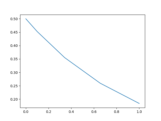
def f(u,p,t):
return -u
u0 = 0.5
tspan = (0., 1.)
prob = de.ODEProblem(f, u0, tspan)
sol = de.solve(prob)
```
The solution object is the same as the one described
[in the DiffEq tutorials](http://diffeq.sciml.ai/dev/tutorials/ode_example#Step-3:-Analyzing-the-Solution-1)
and in the [solution handling documentation](http://diffeq.sciml.ai/dev/basics/solution)
(note: the array interface is missing). Thus for example the solution time points
are saved in `sol.t` and the solution values are saved in `sol.u`. Additionally,
the interpolation `sol(t)` gives a continuous solution.
We can plot the solution values using matplotlib:
```py
import matplotlib.pyplot as plt
plt.plot(sol.t,sol.u)
plt.show()
```
We can utilize the interpolation to get a finer solution:
```py
import numpy
t = numpy.linspace(0,1,100)
u = sol(t)
plt.plot(t,u)
plt.show()
```

### Solve commands
The [common interface arguments](http://diffeq.sciml.ai/dev/basics/common_solver_opts)
can be used to control the solve command. For example, let's use `saveat` to
save the solution at every `t=0.1`, and let's utilize the `Vern9()` 9th order
Runge-Kutta method along with low tolerances `abstol=reltol=1e-10`:
```py
sol = de.solve(prob,de.Vern9(),saveat=0.1,abstol=1e-10,reltol=1e-10)
```
The set of algorithms for ODEs is described
[at the ODE solvers page](http://diffeq.sciml.ai/dev/solvers/ode_solve).
### Compilation with `de.jit` and Julia
When solving a differential equation, it's pertinent that your derivative
function `f` is fast since it occurs in the inner loop of the solver. We can
convert the entire ode problem to symbolic form, optimize that symbolic form,
and emit efficient native code to simulate it using `de.jit` to improve the
efficiency of the solver at the expense of added setup time:
```py
fast_prob = de.jit(prob)
sol = de.solve(fast_prob)
```
Additionally, you can directly define the functions in Julia. This will also
allow for specialization and could be helpful to increase the efficiency for
repeat or long calls. This is done via `seval`:
```py
jul_f = de.seval("(u,p,t)->-u") # Define the anonymous function in Julia
prob = de.ODEProblem(jul_f, u0, tspan)
sol = de.solve(prob)
```
#### Limitations
`de.jit`, uses ModelingToolkit.jl's `modelingtoolkitize` internally and some
restrictions apply. Not all models can be jitted. See the
[`modelingtoolkitize` documentation](https://docs.sciml.ai/ModelingToolkit/stable/tutorials/modelingtoolkitize/#What-is-modelingtoolkitize?)
for more info.
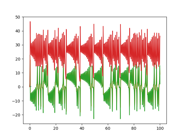
### Systems of ODEs: Lorenz Equations
To solve systems of ODEs, simply use an array as your initial condition and
define `f` as an array function:
```py
def f(u,p,t):
x, y, z = u
sigma, rho, beta = p
return [sigma * (y - x), x * (rho - z) - y, x * y - beta * z]
u0 = [1.0,0.0,0.0]
tspan = (0., 100.)
p = [10.0,28.0,8/3]
prob = de.ODEProblem(f, u0, tspan, p)
sol = de.solve(prob,saveat=0.01)
plt.plot(sol.t,de.transpose(de.stack(sol.u)))
plt.show()
```
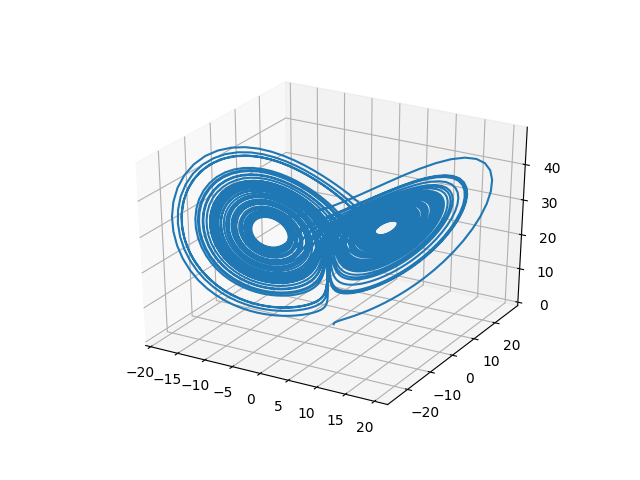
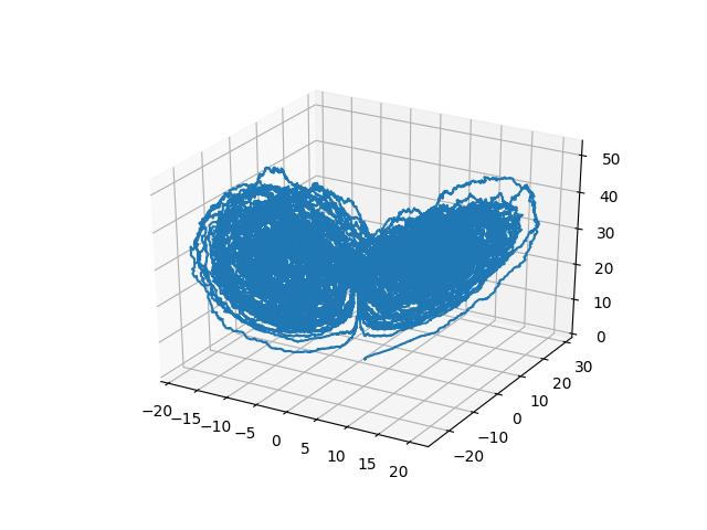
or we can draw the phase plot:
```py
us = de.stack(sol.u)
from mpl_toolkits.mplot3d import Axes3D
fig = plt.figure()
ax = fig.add_subplot(111, projection='3d')
ax.plot(us[0,:],us[1,:],us[2,:])
plt.show()
```
### In-Place Mutating Form
When dealing with systems of equations, in many cases it's helpful to reduce
memory allocations by using mutating functions. In diffeqpy, the mutating
form adds the mutating vector to the front. Let's make a fast version of the
Lorenz derivative, i.e. mutating and JIT compiled:
```py
def f(du,u,p,t):
x, y, z = u
sigma, rho, beta = p
du[0] = sigma * (y - x)
du[1] = x * (rho - z) - y
du[2] = x * y - beta * z
u0 = [1.0,0.0,0.0]
tspan = (0., 100.)
p = [10.0,28.0,2.66]
prob = de.ODEProblem(f, u0, tspan, p)
jit_prob = de.jit(prob)
sol = de.solve(jit_prob)
```
or using a Julia function:
```py
jul_f = de.seval("""
function f(du,u,p,t)
x, y, z = u
sigma, rho, beta = p
du[1] = sigma * (y - x)
du[2] = x * (rho - z) - y
du[3] = x * y - beta * z
end""")
u0 = [1.0,0.0,0.0]
tspan = (0., 100.)
p = [10.0,28.0,2.66]
prob = de.ODEProblem(jul_f, u0, tspan, p)
sol = de.solve(prob)
```
## Stochastic Differential Equation (SDE) Examples
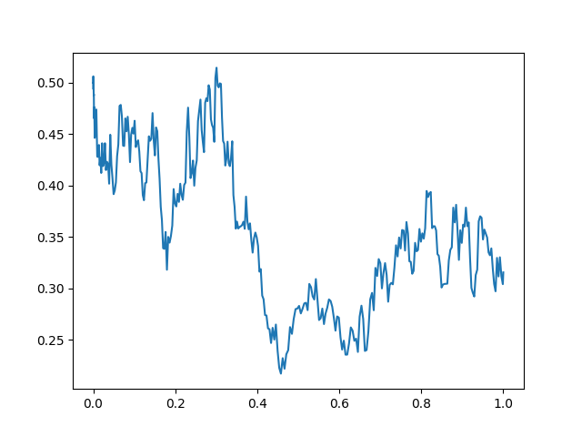
### One-dimensional SDEs
Solving one-dimensonal SDEs `du = f(u,t)dt + g(u,t)dW_t` is like an ODE except
with an extra function for the diffusion (randomness or noise) term. The steps
follow the [SDE tutorial](http://diffeq.sciml.ai/dev/tutorials/sde_example).
```py
def f(u,p,t):
return 1.01*u
def g(u,p,t):
return 0.87*u
u0 = 0.5
tspan = (0.0,1.0)
prob = de.SDEProblem(f,g,u0,tspan)
sol = de.solve(prob,reltol=1e-3,abstol=1e-3)
plt.plot(sol.t,de.stack(sol.u))
plt.show()
```
### Systems of SDEs with Diagonal Noise
An SDE with diagonal noise is where a different Wiener process is applied to
every part of the system. This is common for models with phenomenological noise.
Let's add multiplicative noise to the Lorenz equation:
```py
def f(du,u,p,t):
x, y, z = u
sigma, rho, beta = p
du[0] = sigma * (y - x)
du[1] = x * (rho - z) - y
du[2] = x * y - beta * z
def g(du,u,p,t):
du[0] = 0.3*u[0]
du[1] = 0.3*u[1]
du[2] = 0.3*u[2]
u0 = [1.0,0.0,0.0]
tspan = (0., 100.)
p = [10.0,28.0,2.66]
prob = de.jit(de.SDEProblem(f, g, u0, tspan, p))
sol = de.solve(prob)
# Now let's draw a phase plot
us = de.stack(sol.u)
from mpl_toolkits.mplot3d import Axes3D
fig = plt.figure()
ax = fig.add_subplot(111, projection='3d')
ax.plot(us[0,:],us[1,:],us[2,:])
plt.show()
```
### Systems of SDEs with Non-Diagonal Noise
In many cases you may want to share noise terms across the system. This is
known as non-diagonal noise. The
[DifferentialEquations.jl SDE Tutorial](http://diffeq.sciml.ai/dev/tutorials/sde_example#Example-4:-Systems-of-SDEs-with-Non-Diagonal-Noise-1)
explains how the matrix form of the diffusion term corresponds to the
summation style of multiple Wiener processes. Essentially, the row corresponds
to which system the term is applied to, and the column is which noise term.
So `du[i,j]` is the amount of noise due to the `j`th Wiener process that's
applied to `u[i]`. We solve the Lorenz system with correlated noise as follows:
```py
def f(du,u,p,t):
x, y, z = u
sigma, rho, beta = p
du[0] = sigma * (y - x)
du[1] = x * (rho - z) - y
du[2] = x * y - beta * z
def g(du,u,p,t):
du[0,0] = 0.3*u[0]
du[1,0] = 0.6*u[0]
du[2,0] = 0.2*u[0]
du[0,1] = 1.2*u[1]
du[1,1] = 0.2*u[1]
du[2,1] = 0.3*u[1]
u0 = [1.0,0.0,0.0]
tspan = (0.0,100.0)
p = [10.0,28.0,2.66]
nrp = numpy.zeros((3,2))
prob = de.SDEProblem(f,g,u0,tspan,p,noise_rate_prototype=nrp)
jit_prob = de.jit(prob)
sol = de.solve(jit_prob,saveat=0.005)
# Now let's draw a phase plot
us = de.stack(sol.u)
from mpl_toolkits.mplot3d import Axes3D
fig = plt.figure()
ax = fig.add_subplot(111, projection='3d')
ax.plot(us[0,:],us[1,:],us[2,:])
plt.show()
```
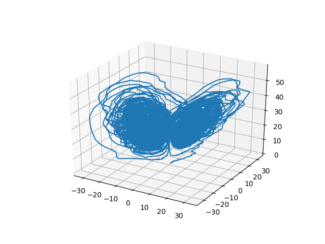
Here you can see that the warping effect of the noise correlations is quite visible!
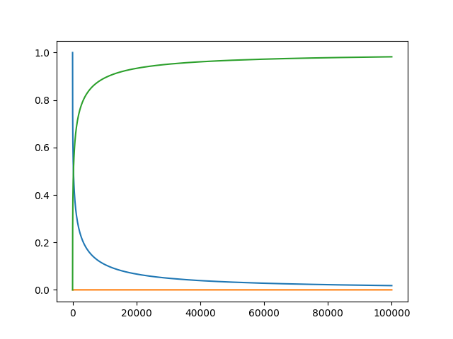
## Differential-Algebraic Equation (DAE) Examples
A differential-algebraic equation is defined by an implicit function
`f(du,u,p,t)=0`. All of the controls are the same as the other examples, except
here you define a function which returns the residuals for each part of the
equation to define the DAE. The initial value `u0` and the initial derivative
`du0` are required, though they do not necessarily have to satisfy `f` (known
as inconsistent initial conditions). The methods will automatically find
consistent initial conditions. In order for this to occur, `differential_vars`
must be set. This vector states which of the variables are differential (have a
derivative term), with `false` meaning that the variable is purely algebraic.
This example shows how to solve the Robertson equation:
```py
def f(du,u,p,t):
resid1 = - 0.04*u[0] + 1e4*u[1]*u[2] - du[0]
resid2 = + 0.04*u[0] - 3e7*u[1]**2 - 1e4*u[1]*u[2] - du[1]
resid3 = u[0] + u[1] + u[2] - 1.0
return [resid1,resid2,resid3]
u0 = [1.0, 0.0, 0.0]
du0 = [-0.04, 0.04, 0.0]
tspan = (0.0,100000.0)
differential_vars = [True,True,False]
prob = de.DAEProblem(f,du0,u0,tspan,differential_vars=differential_vars)
sol = de.solve(prob)
```
and the in-place JIT compiled form:
```py
def f(resid,du,u,p,t):
resid[0] = - 0.04*u[0] + 1e4*u[1]*u[2] - du[0]
resid[1] = + 0.04*u[0] - 3e7*u[1]**2 - 1e4*u[1]*u[2] - du[1]
resid[2] = u[0] + u[1] + u[2] - 1.0
prob = de.DAEProblem(f,du0,u0,tspan,differential_vars=differential_vars)
jit_prob = de.jit(prob) # Error: no method matching matching modelingtoolkitize(::SciMLBase.DAEProblem{...})
sol = de.solve(jit_prob)
```
## Mass Matrices, Sparse Arrays, and More
Mass matrix DAEs, along with many other forms, can be handled by doing an explicit conversion to the Julia types.
See [the PythonCall module's documentation for more details](https://juliapy.github.io/PythonCall.jl/stable/juliacall/).
As an example, let's convert [the mass matrix ODE tutorial in diffeqpy](https://docs.sciml.ai/DiffEqDocs/stable/tutorials/dae_example/).
To do this, the one aspect we need to handle is the conversion of the mass matrix in to a Julia array object. This is done as follows:
```py
from diffeqpy import de
from juliacall import Main as jl
import numpy as np
def rober(du, u, p, t):
y1, y2, y3 = u
k1, k2, k3 = p
du[0] = -k1 * y1 + k3 * y2 * y3
du[1] = k1 * y1 - k3 * y2 * y3 - k2 * y2**2
du[2] = y1 + y2 + y3 - 1
return
M = np.array([[1.0,0.0,0.0],[0.0,1.0,0.0],[0.0,0.0,0.0]])
f = de.ODEFunction(rober, mass_matrix = jl.convert(jl.Array,M))
prob_mm = de.ODEProblem(f, [1.0, 0.0, 0.0], (0.0, 1e5), (0.04, 3e7, 1e4))
sol = de.solve(prob_mm, de.Rodas5P(), reltol = 1e-8, abstol = 1e-8)
```
Notice the only addition is to create the `np.array` object and to perform the manual conversion via `jl.convert(jl.Array,M)` to receive the
Julia `Array` object. This can be done in any case where diffeqpy is not adequately auto-converting to the right Julia type. In some cases this
can be used to improve performance, though here we do it simply for compatability.
Similarly, sparse matrices can be passed in much the same way. For example:
```py
import scipy
spM = scipy.sparse.csr_array(M)
jl.seval("using SparseArrays")
f = de.ODEFunction(rober, mass_matrix = jl.convert(jl.SparseMatrixCSC,M))
prob_mm = de.ODEProblem(f, [1.0, 0.0, 0.0], (0.0, 1e5), (0.04, 3e7, 1e4))
sol = de.solve(prob_mm, de.Rodas5P(), reltol = 1e-8, abstol = 1e-8)
```
## Delay Differential Equations
A delay differential equation is an ODE which allows the use of previous values.
In this case, the function needs to be a JIT compiled Julia function. It looks
just like the ODE, except in this case there is a function `h(p,t)` which allows
you to interpolate and grab previous values.
We must provide a history function `h(p,t)` that gives values for `u` before `t0`.
Here we assume that the solution was constant before the initial time point.
Additionally, we pass `constant_lags = [20.0]` to tell the solver that only
constant-time lags were used and what the lag length was. This helps improve
the solver accuracy by accurately stepping at the points of discontinuity.
Together this is:
```py
f = de.seval("""
function f(du, u, h, p, t)
du[1] = 1.1/(1 + sqrt(10)*(h(p, t-20)[1])^(5/4)) - 10*u[1]/(1 + 40*u[2])
du[2] = 100*u[1]/(1 + 40*u[2]) - 2.43*u[2]
end""")
u0 = [1.05767027/3, 1.030713491/3]
h = de.seval("""
function h(p,t)
[1.05767027/3, 1.030713491/3]
end
""")
tspan = (0.0, 100.0)
constant_lags = [20.0]
prob = de.DDEProblem(f,u0,h,tspan,constant_lags=constant_lags)
sol = de.solve(prob,saveat=0.1)
u1 = [sol.u[i][0] for i in range(0,len(sol.u))]
u2 = [sol.u[i][1] for i in range(0,len(sol.u))]
import matplotlib.pyplot as plt
plt.plot(sol.t,u1)
plt.plot(sol.t,u2)
plt.show()
```
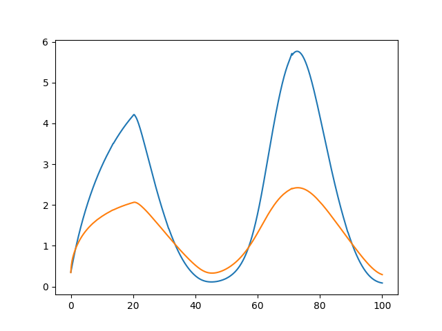
Notice that the solver accurately is able to simulate the kink (discontinuity)
at `t=20` due to the discontinuity of the derivative at the initial time point!
This is why declaring discontinuities can enhance the solver accuracy.
## GPU-Accelerated ODE Solving of Ensembles
In many cases one is interested in solving the same ODE many times over many
different initial conditions and parameters. In diffeqpy parlance this is called
an ensemble solve. diffeqpy inherits the parallelism tools of the
[SciML ecosystem](https://sciml.ai/) that are used for things like
[automated equation discovery and acceleration](https://arxiv.org/abs/2001.04385).
Here we will demonstrate using these parallel tools to accelerate the solving
of an ensemble.
First, let's define the JIT-accelerated Lorenz equation like before:
```py
from diffeqpy import de
def f(u,p,t):
x, y, z = u
sigma, rho, beta = p
return [sigma * (y - x), x * (rho - z) - y, x * y - beta * z]
u0 = [1.0,0.0,0.0]
tspan = (0., 100.)
p = [10.0,28.0,8/3]
prob = de.ODEProblem(f, u0, tspan, p)
fast_prob = de.jit32(prob)
sol = de.solve(fast_prob,saveat=0.01)
```
Note that here we used `de.jit32` to JIT-compile the problem into a `Float32` form in order to make it more
efficient on most GPUs.
Now we use the `EnsembleProblem` as defined on the
[ensemble parallelism page of the documentation](https://diffeq.sciml.ai/stable/features/ensemble/):
Let's build an ensemble by utilizing uniform random numbers to randomize the
initial conditions and parameters:
```py
import random
def prob_func(prob,i,rep):
return de.remake(prob,u0=[random.uniform(0, 1)*u0[i] for i in range(0,3)],
p=[random.uniform(0, 1)*p[i] for i in range(0,3)])
ensembleprob = de.EnsembleProblem(fast_prob, prob_func=prob_func, safetycopy=False)
```
Now we solve the ensemble in serial:
```py
sol = de.solve(ensembleprob,de.Tsit5(),de.EnsembleSerial(),trajectories=10000,saveat=0.01)
```
To add GPUs to the mix, we need to bring in [DiffEqGPU](https://github.com/SciML/DiffEqGPU.jl).
The command `from diffeqpy import cuda` will install CUDA for you and bring all of the bindings into the returned object:
#### Note: `from diffeqpy import cuda` can take awhile to run the first time as it installs the drivers!
Now we simply use `EnsembleGPUKernel(cuda.CUDABackend())` with a
GPU-specialized ODE solver `cuda.GPUTsit5()` to solve 10,000 ODEs on the GPU in
parallel:
```py
sol = de.solve(ensembleprob,cuda.GPUTsit5(),cuda.EnsembleGPUKernel(cuda.CUDABackend()),trajectories=10000,saveat=0.01)
```
For the full list of choices for specialized GPU solvers, see
[the DiffEqGPU.jl documentation](https://docs.sciml.ai/DiffEqGPU/stable/manual/ensemblegpukernel/).
Note that `EnsembleGPUArray` can be used as well, like:
```py
sol = de.solve(ensembleprob,de.Tsit5(),cuda.EnsembleGPUArray(cuda.CUDABackend()),trajectories=10000,saveat=0.01)
```
though we highly recommend the `EnsembleGPUKernel` methods for more speed. Given
the way the JIT compilation performed will also ensure that the faster kernel
generation methods work, `EnsembleGPUKernel` is almost certainly the
better choice in most applications.
### Benchmark
To see how much of an effect the parallelism has, let's test this against R's
deSolve package. This is exactly the same problem as the documentation example
for deSolve, so let's copy that verbatim and then add a function to do the
ensemble generation:
```py
import numpy as np
from scipy.integrate import odeint
def lorenz(state, t, sigma, beta, rho):
x, y, z = state
dx = sigma * (y - x)
dy = x * (rho - z) - y
dz = x * y - beta * z
return [dx, dy, dz]
sigma = 10.0
beta = 8.0 / 3.0
rho = 28.0
p = (sigma, beta, rho)
y0 = [1.0, 1.0, 1.0]
t = np.arange(0.0, 100.0, 0.01)
result = odeint(lorenz, y0, t, p)
```
Using `lapply` to generate the ensemble we get:
```py
import timeit
def time_func():
for itr in range(1, 1001):
result = odeint(lorenz, y0, t, p)
timeit.Timer(time_func).timeit(number=1)
# 38.08861699999761 seconds
```
Now let's see how the JIT-accelerated serial Julia version stacks up against that:
```py
def time_func():
sol = de.solve(ensembleprob,de.Tsit5(),de.EnsembleSerial(),trajectories=1000,saveat=0.01)
timeit.Timer(time_func).timeit(number=1)
# 3.1903300999983912
```
Julia is already about 12x faster than the pure Python solvers here! Now let's add
GPU-acceleration to the mix:
```py
def time_func():
sol = de.solve(ensembleprob,cuda.GPUTsit5(),cuda.EnsembleGPUKernel(cuda.CUDABackend()),trajectories=1000,saveat=0.01)
timeit.Timer(time_func).timeit(number=1)
# 0.013322799997695256
```
Already 2900x faster than SciPy! But the GPU acceleration is made for massively
parallel problems, so let's up the trajectories a bit. We will not use more
trajectories from R because that would take too much computing power, so let's
see what happens to the Julia serial and GPU at 10,000 trajectories:
```py
def time_func():
sol = de.solve(ensembleprob,de.Tsit5(),de.EnsembleSerial(),trajectories=10000,saveat=0.01)
timeit.Timer(time_func).timeit(number=1)
# 68.80795999999827
```
```py
def time_func():
sol = de.solve(ensembleprob,cuda.GPUTsit5(),cuda.EnsembleGPUKernel(cuda.CUDABackend()),trajectories=10000,saveat=0.01)
timeit.Timer(time_func).timeit(number=1)
# 0.10774460000175168
```
To compare this to the pure Julia code:
```julia
using OrdinaryDiffEq, DiffEqGPU, CUDA, StaticArrays
function lorenz(u, p, t)
σ = p[1]
ρ = p[2]
β = p[3]
du1 = σ * (u[2] - u[1])
du2 = u[1] * (ρ - u[3]) - u[2]
du3 = u[1] * u[2] - β * u[3]
return SVector{3}(du1, du2, du3)
end
u0 = SA[1.0f0; 0.0f0; 0.0f0]
tspan = (0.0f0, 10.0f0)
p = SA[10.0f0, 28.0f0, 8 / 3.0f0]
prob = ODEProblem{false}(lorenz, u0, tspan, p)
prob_func = (prob, i, repeat) -> remake(prob, p = (@SVector rand(Float32, 3)) .* p)
monteprob = EnsembleProblem(prob, prob_func = prob_func, safetycopy = false)
@time sol = solve(monteprob, GPUTsit5(), EnsembleGPUKernel(CUDA.CUDABackend()),
trajectories = 10_000,
saveat = 0.01);
# 0.014481 seconds (257.64 k allocations: 13.130 MiB)
```
which is about an order of magnitude faster for computing 10,000 trajectories,
note that the major factors are that we cannot define 32-bit floating point values
from Python and the `prob_func` for generating the initial conditions and parameters
is a major bottleneck since this function is written in Python.
To see how this scales in Julia, let's take it to insane heights. First, let's
reduce the amount we're saving:
```julia
@time sol = solve(monteprob,GPUTsit5(),EnsembleGPUKernel(CUDA.CUDABackend()),trajectories=10_000,saveat=1.0f0)
0.015040 seconds (257.64 k allocations: 13.130 MiB)
```
This highlights that controlling memory pressure is key with GPU usage: you will
get much better performance when requiring less saved points on the GPU.
```julia
@time sol = solve(monteprob,GPUTsit5(),EnsembleGPUKernel(CUDA.CUDABackend()),trajectories=100_000,saveat=1.0f0)
# 0.150901 seconds (2.60 M allocations: 131.576 MiB)
```
compared to serial:
```julia
@time sol = solve(monteprob,Tsit5(),EnsembleSerial(),trajectories=100_000,saveat=1.0f0)
# 22.136743 seconds (16.40 M allocations: 1.628 GiB, 42.98% gc time)
```
And now we start to see that scaling power! Let's solve 1 million trajectories:
```julia
@time sol = solve(monteprob,GPUTsit5(),EnsembleGPUKernel(CUDA.CUDABackend()),trajectories=1_000_000,saveat=1.0f0)
# 1.031295 seconds (3.40 M allocations: 241.075 MiB)
```
For reference, let's look at deSolve with the change to only save that much:
```py
t = np.arange(0.0, 100.0, 1.0)
def time_func():
for itr in range(1, 1001):
result = odeint(lorenz, y0, t, p)
timeit.Timer(time_func).timeit(number=1)
# 37.42609280000033
```
The GPU version is solving 1000x as many trajectories, 37x as fast! So conclusion,
if you need the most speed, you may want to move to the Julia version to get the
most out of your GPU due to Float32's, and when using GPUs make sure it's a problem
with a relatively average or low memory pressure, and these methods will give
orders of magnitude acceleration compared to what you might be used to.
## GPU Backend Choices
Just like DiffEqGPU.jl, diffeqpy supports many different GPU venders. `from diffeqpy import cuda`
is just for cuda, but the following others are supported:
- `from diffeqpy import cuda` with `cuda.CUDABackend` for NVIDIA GPUs via CUDA
- `from diffeqpy import amdgpu` with `amdgpu.AMDGPUBackend` for AMD GPUs
- `from diffeqpy import oneapi` with `oneapi.oneAPIBackend` for Intel's oneAPI GPUs
- `from diffeqpy import metal` with `metal.MetalBackend` for Apple's Metal GPUs (on M-series processors)
For more information, see [the DiffEqGPU.jl documentation](https://docs.sciml.ai/DiffEqGPU/stable/manual/backends/).
## Known Limitations
- Autodiff does not work on Python functions. When applicable, either define the derivative function
as a Julia function or set the algorithm to use finite differencing, i.e. `Rodas5(autodiff=false)`.
All default methods use autodiff.
- Delay differential equations have to use Julia-defined functions otherwise the history function is
not appropriately typed with the overloads.
## Testing
Unit tests can be run by [`tox`](http://tox.readthedocs.io).
```sh
tox
```
### Troubleshooting
In case you encounter silent failure from `tox`, try running it with
`-- -s` (e.g., `tox -e py36 -- -s`) where `-s` option (`--capture=no`,
i.e., don't capture stdio) is passed to `py.test`. It may show an
error message `"error initializing LibGit2 module"`. In this case,
setting environment variable `SSL_CERT_FILE` may help; e.g., try:
```sh
SSL_CERT_FILE=PATH/TO/cert.pem tox -e py36
```
See also: [julia#18693](https://github.com/JuliaLang/julia/issues/18693).
Raw data
{
"_id": null,
"home_page": "http://github.com/SciML/diffeqpy",
"name": "diffeqpy",
"maintainer": null,
"docs_url": null,
"requires_python": null,
"maintainer_email": null,
"keywords": "differential equations stochastic ordinary delay differential-algebraic dae ode sde dde oneapi AMD ROCm CUDA Metal GPU",
"author": "Chris Rackauckas and Takafumi Arakaki",
"author_email": "contact@sciml.ai",
"download_url": "https://files.pythonhosted.org/packages/56/68/e9ec32f94718839ab3079808236e058493229de9ad9cde0bebff932f347b/diffeqpy-2.5.4.tar.gz",
"platform": null,
"description": "# diffeqpy\n\n[](https://gitter.im/JuliaDiffEq/Lobby?utm_source=badge&utm_medium=badge&utm_campaign=pr-badge&utm_content=badge)\n[](https://github.com/SciML/diffeqpy/actions)\n\ndiffeqpy is a package for solving differential equations in Python. It utilizes\n[DifferentialEquations.jl](http://diffeq.sciml.ai/dev/) for its core routines\nto give high performance solving of many different types of differential equations,\nincluding:\n\n- Discrete equations (function maps, discrete stochastic (Gillespie/Markov)\n simulations)\n- Ordinary differential equations (ODEs)\n- Split and Partitioned ODEs (Symplectic integrators, IMEX Methods)\n- Stochastic ordinary differential equations (SODEs or SDEs)\n- Random differential equations (RODEs or RDEs)\n- Differential algebraic equations (DAEs)\n- Delay differential equations (DDEs)\n- Mixed discrete and continuous equations (Hybrid Equations, Jump Diffusions)\n\ndirectly in Python.\n\nIf you have any questions, or just want to chat about solvers/using the package,\nplease feel free to chat in the [Gitter channel](https://gitter.im/JuliaDiffEq/Lobby?utm_source=badge&utm_medium=badge&utm_campaign=pr-badge&utm_content=badge). For bug reports, feature requests, etc., please submit an issue.\n\n## Installation\n\nTo install diffeqpy, use pip:\n\n```\npip install diffeqpy\n```\n\nand you're good!\n\n## Collab Notebook Examples\n\n- [Solving the Lorenz equation faster than SciPy+Numba](https://colab.research.google.com/drive/1SQCu1puMQO01i3oMg0TXfa1uf7BqgsEW?usp=sharing)\n- [Solving ODEs on GPUs Fast in Python with diffeqpy](https://colab.research.google.com/drive/1bnQMdNvg0AL-LyPcXBiH10jBij5QUmtY?usp=sharing)\n\n## General Flow\n\nImport and setup the solvers available in *DifferentialEquations.jl* via the command:\n\n```py\nfrom diffeqpy import de\n```\nIn case only the solvers available in *OrdinaryDiffEq.jl* are required then use the command:\n```py\nfrom diffeqpy import ode\n```\nThe general flow for using the package is to follow exactly as would be done\nin Julia, except add `de.` or `ode.` in front. Note that `ode.` has lesser loading time and a smaller memory footprint compared to `de.`.\nMost of the commands will work without any modification. Thus\n[the DifferentialEquations.jl documentation](https://github.com/SciML/DifferentialEquations.jl)\nand the [DiffEqTutorials](https://github.com/SciML/DiffEqTutorials.jl)\nare the main in-depth documentation for this package. Below we will show how to\ntranslate these docs to Python code.\n\n## Note about !\n\nPython does not allow `!` in function names, so this is also [a limitation of pyjulia](https://pyjulia.readthedocs.io/en/latest/limitations.html#mismatch-in-valid-set-of-identifiers)\nTo use functions which on the Julia side have a `!`, like `step!`, replace `!` by `_b`, for example:\n\n```py\nfrom diffeqpy import de\n\ndef f(u,p,t):\n return -u\n\nu0 = 0.5\ntspan = (0., 1.)\nprob = de.ODEProblem(f, u0, tspan)\nintegrator = de.init(prob, de.Tsit5())\nde.step_b(integrator)\n```\n\nis valid Python code for using [the integrator interface](https://diffeq.sciml.ai/stable/basics/integrator/).\n\n\n## Ordinary Differential Equation (ODE) Examples\n\n### One-dimensional ODEs\n\n```py\nfrom diffeqpy import de\n\ndef f(u,p,t):\n return -u\n\nu0 = 0.5\ntspan = (0., 1.)\nprob = de.ODEProblem(f, u0, tspan)\nsol = de.solve(prob)\n```\n\nThe solution object is the same as the one described\n[in the DiffEq tutorials](http://diffeq.sciml.ai/dev/tutorials/ode_example#Step-3:-Analyzing-the-Solution-1)\nand in the [solution handling documentation](http://diffeq.sciml.ai/dev/basics/solution)\n(note: the array interface is missing). Thus for example the solution time points\nare saved in `sol.t` and the solution values are saved in `sol.u`. Additionally,\nthe interpolation `sol(t)` gives a continuous solution.\n\nWe can plot the solution values using matplotlib:\n\n```py\nimport matplotlib.pyplot as plt\nplt.plot(sol.t,sol.u)\nplt.show()\n```\n\n\n\nWe can utilize the interpolation to get a finer solution:\n\n```py\nimport numpy\nt = numpy.linspace(0,1,100)\nu = sol(t)\nplt.plot(t,u)\nplt.show()\n```\n\n\n\n### Solve commands\n\nThe [common interface arguments](http://diffeq.sciml.ai/dev/basics/common_solver_opts)\ncan be used to control the solve command. For example, let's use `saveat` to\nsave the solution at every `t=0.1`, and let's utilize the `Vern9()` 9th order\nRunge-Kutta method along with low tolerances `abstol=reltol=1e-10`:\n\n```py\nsol = de.solve(prob,de.Vern9(),saveat=0.1,abstol=1e-10,reltol=1e-10)\n```\n\nThe set of algorithms for ODEs is described\n[at the ODE solvers page](http://diffeq.sciml.ai/dev/solvers/ode_solve).\n\n### Compilation with `de.jit` and Julia\n\nWhen solving a differential equation, it's pertinent that your derivative\nfunction `f` is fast since it occurs in the inner loop of the solver. We can\nconvert the entire ode problem to symbolic form, optimize that symbolic form,\nand emit efficient native code to simulate it using `de.jit` to improve the\nefficiency of the solver at the expense of added setup time:\n\n```py\nfast_prob = de.jit(prob)\nsol = de.solve(fast_prob)\n```\n\nAdditionally, you can directly define the functions in Julia. This will also\nallow for specialization and could be helpful to increase the efficiency for\nrepeat or long calls. This is done via `seval`:\n\n```py\njul_f = de.seval(\"(u,p,t)->-u\") # Define the anonymous function in Julia\nprob = de.ODEProblem(jul_f, u0, tspan)\nsol = de.solve(prob)\n```\n\n#### Limitations\n\n`de.jit`, uses ModelingToolkit.jl's `modelingtoolkitize` internally and some\nrestrictions apply. Not all models can be jitted. See the\n[`modelingtoolkitize` documentation](https://docs.sciml.ai/ModelingToolkit/stable/tutorials/modelingtoolkitize/#What-is-modelingtoolkitize?)\nfor more info.\n\n### Systems of ODEs: Lorenz Equations\n\nTo solve systems of ODEs, simply use an array as your initial condition and\ndefine `f` as an array function:\n\n```py\ndef f(u,p,t):\n x, y, z = u\n sigma, rho, beta = p\n return [sigma * (y - x), x * (rho - z) - y, x * y - beta * z]\n\nu0 = [1.0,0.0,0.0]\ntspan = (0., 100.)\np = [10.0,28.0,8/3]\nprob = de.ODEProblem(f, u0, tspan, p)\nsol = de.solve(prob,saveat=0.01)\n\nplt.plot(sol.t,de.transpose(de.stack(sol.u)))\nplt.show()\n```\n\n\n\nor we can draw the phase plot:\n\n```py\nus = de.stack(sol.u)\nfrom mpl_toolkits.mplot3d import Axes3D\nfig = plt.figure()\nax = fig.add_subplot(111, projection='3d')\nax.plot(us[0,:],us[1,:],us[2,:])\nplt.show()\n```\n\n\n\n### In-Place Mutating Form\n\nWhen dealing with systems of equations, in many cases it's helpful to reduce\nmemory allocations by using mutating functions. In diffeqpy, the mutating\nform adds the mutating vector to the front. Let's make a fast version of the\nLorenz derivative, i.e. mutating and JIT compiled:\n\n```py\ndef f(du,u,p,t):\n x, y, z = u\n sigma, rho, beta = p\n du[0] = sigma * (y - x)\n du[1] = x * (rho - z) - y\n du[2] = x * y - beta * z\n\nu0 = [1.0,0.0,0.0]\ntspan = (0., 100.)\np = [10.0,28.0,2.66]\nprob = de.ODEProblem(f, u0, tspan, p)\njit_prob = de.jit(prob)\nsol = de.solve(jit_prob)\n```\n\nor using a Julia function:\n\n```py\njul_f = de.seval(\"\"\"\nfunction f(du,u,p,t)\n x, y, z = u\n sigma, rho, beta = p\n du[1] = sigma * (y - x)\n du[2] = x * (rho - z) - y\n du[3] = x * y - beta * z\nend\"\"\")\nu0 = [1.0,0.0,0.0]\ntspan = (0., 100.)\np = [10.0,28.0,2.66]\nprob = de.ODEProblem(jul_f, u0, tspan, p)\nsol = de.solve(prob)\n```\n\n## Stochastic Differential Equation (SDE) Examples\n\n### One-dimensional SDEs\n\nSolving one-dimensonal SDEs `du = f(u,t)dt + g(u,t)dW_t` is like an ODE except\nwith an extra function for the diffusion (randomness or noise) term. The steps\nfollow the [SDE tutorial](http://diffeq.sciml.ai/dev/tutorials/sde_example).\n\n```py\ndef f(u,p,t):\n return 1.01*u\n\ndef g(u,p,t):\n return 0.87*u\n\nu0 = 0.5\ntspan = (0.0,1.0)\nprob = de.SDEProblem(f,g,u0,tspan)\nsol = de.solve(prob,reltol=1e-3,abstol=1e-3)\n\nplt.plot(sol.t,de.stack(sol.u))\nplt.show()\n```\n\n\n\n### Systems of SDEs with Diagonal Noise\n\nAn SDE with diagonal noise is where a different Wiener process is applied to\nevery part of the system. This is common for models with phenomenological noise.\nLet's add multiplicative noise to the Lorenz equation:\n\n```py\ndef f(du,u,p,t):\n x, y, z = u\n sigma, rho, beta = p\n du[0] = sigma * (y - x)\n du[1] = x * (rho - z) - y\n du[2] = x * y - beta * z\n\ndef g(du,u,p,t):\n du[0] = 0.3*u[0]\n du[1] = 0.3*u[1]\n du[2] = 0.3*u[2]\n\nu0 = [1.0,0.0,0.0]\ntspan = (0., 100.)\np = [10.0,28.0,2.66]\nprob = de.jit(de.SDEProblem(f, g, u0, tspan, p))\nsol = de.solve(prob)\n\n# Now let's draw a phase plot\n\nus = de.stack(sol.u)\nfrom mpl_toolkits.mplot3d import Axes3D\nfig = plt.figure()\nax = fig.add_subplot(111, projection='3d')\nax.plot(us[0,:],us[1,:],us[2,:])\nplt.show()\n```\n\n\n\n### Systems of SDEs with Non-Diagonal Noise\n\nIn many cases you may want to share noise terms across the system. This is\nknown as non-diagonal noise. The\n[DifferentialEquations.jl SDE Tutorial](http://diffeq.sciml.ai/dev/tutorials/sde_example#Example-4:-Systems-of-SDEs-with-Non-Diagonal-Noise-1)\nexplains how the matrix form of the diffusion term corresponds to the\nsummation style of multiple Wiener processes. Essentially, the row corresponds\nto which system the term is applied to, and the column is which noise term.\nSo `du[i,j]` is the amount of noise due to the `j`th Wiener process that's\napplied to `u[i]`. We solve the Lorenz system with correlated noise as follows:\n\n```py\ndef f(du,u,p,t):\n x, y, z = u\n sigma, rho, beta = p\n du[0] = sigma * (y - x)\n du[1] = x * (rho - z) - y\n du[2] = x * y - beta * z\n\ndef g(du,u,p,t):\n du[0,0] = 0.3*u[0]\n du[1,0] = 0.6*u[0]\n du[2,0] = 0.2*u[0]\n du[0,1] = 1.2*u[1]\n du[1,1] = 0.2*u[1]\n du[2,1] = 0.3*u[1]\n\n\nu0 = [1.0,0.0,0.0]\ntspan = (0.0,100.0)\np = [10.0,28.0,2.66]\nnrp = numpy.zeros((3,2))\nprob = de.SDEProblem(f,g,u0,tspan,p,noise_rate_prototype=nrp)\njit_prob = de.jit(prob)\nsol = de.solve(jit_prob,saveat=0.005)\n\n# Now let's draw a phase plot\n\nus = de.stack(sol.u)\nfrom mpl_toolkits.mplot3d import Axes3D\nfig = plt.figure()\nax = fig.add_subplot(111, projection='3d')\nax.plot(us[0,:],us[1,:],us[2,:])\nplt.show()\n```\n\n\n\nHere you can see that the warping effect of the noise correlations is quite visible!\n\n## Differential-Algebraic Equation (DAE) Examples\n\nA differential-algebraic equation is defined by an implicit function\n`f(du,u,p,t)=0`. All of the controls are the same as the other examples, except\nhere you define a function which returns the residuals for each part of the\nequation to define the DAE. The initial value `u0` and the initial derivative\n`du0` are required, though they do not necessarily have to satisfy `f` (known\nas inconsistent initial conditions). The methods will automatically find\nconsistent initial conditions. In order for this to occur, `differential_vars`\nmust be set. This vector states which of the variables are differential (have a\nderivative term), with `false` meaning that the variable is purely algebraic.\n\nThis example shows how to solve the Robertson equation:\n\n```py\ndef f(du,u,p,t):\n resid1 = - 0.04*u[0] + 1e4*u[1]*u[2] - du[0]\n resid2 = + 0.04*u[0] - 3e7*u[1]**2 - 1e4*u[1]*u[2] - du[1]\n resid3 = u[0] + u[1] + u[2] - 1.0\n return [resid1,resid2,resid3]\n\nu0 = [1.0, 0.0, 0.0]\ndu0 = [-0.04, 0.04, 0.0]\ntspan = (0.0,100000.0)\ndifferential_vars = [True,True,False]\nprob = de.DAEProblem(f,du0,u0,tspan,differential_vars=differential_vars)\nsol = de.solve(prob)\n```\n\n\n\nand the in-place JIT compiled form:\n\n```py\ndef f(resid,du,u,p,t):\n resid[0] = - 0.04*u[0] + 1e4*u[1]*u[2] - du[0]\n resid[1] = + 0.04*u[0] - 3e7*u[1]**2 - 1e4*u[1]*u[2] - du[1]\n resid[2] = u[0] + u[1] + u[2] - 1.0\n\nprob = de.DAEProblem(f,du0,u0,tspan,differential_vars=differential_vars)\njit_prob = de.jit(prob) # Error: no method matching matching modelingtoolkitize(::SciMLBase.DAEProblem{...})\nsol = de.solve(jit_prob)\n```\n\n## Mass Matrices, Sparse Arrays, and More\n\nMass matrix DAEs, along with many other forms, can be handled by doing an explicit conversion to the Julia types.\nSee [the PythonCall module's documentation for more details](https://juliapy.github.io/PythonCall.jl/stable/juliacall/).\n\nAs an example, let's convert [the mass matrix ODE tutorial in diffeqpy](https://docs.sciml.ai/DiffEqDocs/stable/tutorials/dae_example/).\nTo do this, the one aspect we need to handle is the conversion of the mass matrix in to a Julia array object. This is done as follows:\n\n```py\nfrom diffeqpy import de\nfrom juliacall import Main as jl\nimport numpy as np\n\ndef rober(du, u, p, t):\n y1, y2, y3 = u\n k1, k2, k3 = p\n du[0] = -k1 * y1 + k3 * y2 * y3\n du[1] = k1 * y1 - k3 * y2 * y3 - k2 * y2**2\n du[2] = y1 + y2 + y3 - 1\n return\n\nM = np.array([[1.0,0.0,0.0],[0.0,1.0,0.0],[0.0,0.0,0.0]])\nf = de.ODEFunction(rober, mass_matrix = jl.convert(jl.Array,M))\nprob_mm = de.ODEProblem(f, [1.0, 0.0, 0.0], (0.0, 1e5), (0.04, 3e7, 1e4))\nsol = de.solve(prob_mm, de.Rodas5P(), reltol = 1e-8, abstol = 1e-8)\n```\n\nNotice the only addition is to create the `np.array` object and to perform the manual conversion via `jl.convert(jl.Array,M)` to receive the\nJulia `Array` object. This can be done in any case where diffeqpy is not adequately auto-converting to the right Julia type. In some cases this\ncan be used to improve performance, though here we do it simply for compatability.\n\nSimilarly, sparse matrices can be passed in much the same way. For example:\n\n```py\nimport scipy\nspM = scipy.sparse.csr_array(M)\njl.seval(\"using SparseArrays\")\n\nf = de.ODEFunction(rober, mass_matrix = jl.convert(jl.SparseMatrixCSC,M))\nprob_mm = de.ODEProblem(f, [1.0, 0.0, 0.0], (0.0, 1e5), (0.04, 3e7, 1e4))\nsol = de.solve(prob_mm, de.Rodas5P(), reltol = 1e-8, abstol = 1e-8)\n```\n\n## Delay Differential Equations\n\nA delay differential equation is an ODE which allows the use of previous values.\nIn this case, the function needs to be a JIT compiled Julia function. It looks\njust like the ODE, except in this case there is a function `h(p,t)` which allows\nyou to interpolate and grab previous values.\n\nWe must provide a history function `h(p,t)` that gives values for `u` before `t0`.\nHere we assume that the solution was constant before the initial time point.\nAdditionally, we pass `constant_lags = [20.0]` to tell the solver that only\nconstant-time lags were used and what the lag length was. This helps improve\nthe solver accuracy by accurately stepping at the points of discontinuity.\nTogether this is:\n\n```py\nf = de.seval(\"\"\"\nfunction f(du, u, h, p, t)\n du[1] = 1.1/(1 + sqrt(10)*(h(p, t-20)[1])^(5/4)) - 10*u[1]/(1 + 40*u[2])\n du[2] = 100*u[1]/(1 + 40*u[2]) - 2.43*u[2]\nend\"\"\")\nu0 = [1.05767027/3, 1.030713491/3]\n\nh = de.seval(\"\"\"\nfunction h(p,t)\n [1.05767027/3, 1.030713491/3]\nend\n\"\"\")\n\ntspan = (0.0, 100.0)\nconstant_lags = [20.0]\nprob = de.DDEProblem(f,u0,h,tspan,constant_lags=constant_lags)\nsol = de.solve(prob,saveat=0.1)\n\nu1 = [sol.u[i][0] for i in range(0,len(sol.u))]\nu2 = [sol.u[i][1] for i in range(0,len(sol.u))]\n\nimport matplotlib.pyplot as plt\nplt.plot(sol.t,u1)\nplt.plot(sol.t,u2)\nplt.show()\n```\n\n\n\nNotice that the solver accurately is able to simulate the kink (discontinuity)\nat `t=20` due to the discontinuity of the derivative at the initial time point!\nThis is why declaring discontinuities can enhance the solver accuracy.\n\n## GPU-Accelerated ODE Solving of Ensembles\n\nIn many cases one is interested in solving the same ODE many times over many\ndifferent initial conditions and parameters. In diffeqpy parlance this is called\nan ensemble solve. diffeqpy inherits the parallelism tools of the\n[SciML ecosystem](https://sciml.ai/) that are used for things like\n[automated equation discovery and acceleration](https://arxiv.org/abs/2001.04385).\nHere we will demonstrate using these parallel tools to accelerate the solving\nof an ensemble.\n\nFirst, let's define the JIT-accelerated Lorenz equation like before:\n\n```py\nfrom diffeqpy import de\n\ndef f(u,p,t):\n x, y, z = u\n sigma, rho, beta = p\n return [sigma * (y - x), x * (rho - z) - y, x * y - beta * z]\n\nu0 = [1.0,0.0,0.0]\ntspan = (0., 100.)\np = [10.0,28.0,8/3]\nprob = de.ODEProblem(f, u0, tspan, p)\nfast_prob = de.jit32(prob)\nsol = de.solve(fast_prob,saveat=0.01)\n```\n\nNote that here we used `de.jit32` to JIT-compile the problem into a `Float32` form in order to make it more\nefficient on most GPUs.\n\nNow we use the `EnsembleProblem` as defined on the\n[ensemble parallelism page of the documentation](https://diffeq.sciml.ai/stable/features/ensemble/):\nLet's build an ensemble by utilizing uniform random numbers to randomize the\ninitial conditions and parameters:\n\n```py\nimport random\ndef prob_func(prob,i,rep):\n return de.remake(prob,u0=[random.uniform(0, 1)*u0[i] for i in range(0,3)],\n p=[random.uniform(0, 1)*p[i] for i in range(0,3)])\n\nensembleprob = de.EnsembleProblem(fast_prob, prob_func=prob_func, safetycopy=False)\n```\n\nNow we solve the ensemble in serial:\n\n```py\nsol = de.solve(ensembleprob,de.Tsit5(),de.EnsembleSerial(),trajectories=10000,saveat=0.01)\n```\n\nTo add GPUs to the mix, we need to bring in [DiffEqGPU](https://github.com/SciML/DiffEqGPU.jl).\nThe command `from diffeqpy import cuda` will install CUDA for you and bring all of the bindings into the returned object:\n\n#### Note: `from diffeqpy import cuda` can take awhile to run the first time as it installs the drivers!\n\nNow we simply use `EnsembleGPUKernel(cuda.CUDABackend())` with a\nGPU-specialized ODE solver `cuda.GPUTsit5()` to solve 10,000 ODEs on the GPU in\nparallel:\n\n```py\nsol = de.solve(ensembleprob,cuda.GPUTsit5(),cuda.EnsembleGPUKernel(cuda.CUDABackend()),trajectories=10000,saveat=0.01)\n```\n\nFor the full list of choices for specialized GPU solvers, see\n[the DiffEqGPU.jl documentation](https://docs.sciml.ai/DiffEqGPU/stable/manual/ensemblegpukernel/).\n\nNote that `EnsembleGPUArray` can be used as well, like:\n\n```py\nsol = de.solve(ensembleprob,de.Tsit5(),cuda.EnsembleGPUArray(cuda.CUDABackend()),trajectories=10000,saveat=0.01)\n```\n\nthough we highly recommend the `EnsembleGPUKernel` methods for more speed. Given\nthe way the JIT compilation performed will also ensure that the faster kernel\ngeneration methods work, `EnsembleGPUKernel` is almost certainly the\nbetter choice in most applications.\n\n### Benchmark\n\nTo see how much of an effect the parallelism has, let's test this against R's\ndeSolve package. This is exactly the same problem as the documentation example\nfor deSolve, so let's copy that verbatim and then add a function to do the\nensemble generation:\n\n```py\nimport numpy as np\nfrom scipy.integrate import odeint\n\ndef lorenz(state, t, sigma, beta, rho):\n x, y, z = state\n\n dx = sigma * (y - x)\n dy = x * (rho - z) - y\n dz = x * y - beta * z\n\n return [dx, dy, dz]\n\nsigma = 10.0\nbeta = 8.0 / 3.0\nrho = 28.0\np = (sigma, beta, rho)\ny0 = [1.0, 1.0, 1.0]\n\nt = np.arange(0.0, 100.0, 0.01)\nresult = odeint(lorenz, y0, t, p)\n```\n\nUsing `lapply` to generate the ensemble we get:\n\n```py\nimport timeit\ndef time_func():\n for itr in range(1, 1001):\n result = odeint(lorenz, y0, t, p)\n\ntimeit.Timer(time_func).timeit(number=1)\n\n# 38.08861699999761 seconds\n```\n\nNow let's see how the JIT-accelerated serial Julia version stacks up against that:\n\n```py\ndef time_func():\n sol = de.solve(ensembleprob,de.Tsit5(),de.EnsembleSerial(),trajectories=1000,saveat=0.01)\n\ntimeit.Timer(time_func).timeit(number=1)\n\n# 3.1903300999983912\n```\n\nJulia is already about 12x faster than the pure Python solvers here! Now let's add\nGPU-acceleration to the mix:\n\n```py\ndef time_func():\n sol = de.solve(ensembleprob,cuda.GPUTsit5(),cuda.EnsembleGPUKernel(cuda.CUDABackend()),trajectories=1000,saveat=0.01)\n\ntimeit.Timer(time_func).timeit(number=1)\n\n# 0.013322799997695256\n```\n\nAlready 2900x faster than SciPy! But the GPU acceleration is made for massively\nparallel problems, so let's up the trajectories a bit. We will not use more\ntrajectories from R because that would take too much computing power, so let's\nsee what happens to the Julia serial and GPU at 10,000 trajectories:\n\n```py\ndef time_func():\n sol = de.solve(ensembleprob,de.Tsit5(),de.EnsembleSerial(),trajectories=10000,saveat=0.01)\n\ntimeit.Timer(time_func).timeit(number=1)\n\n# 68.80795999999827\n```\n\n```py\ndef time_func():\n sol = de.solve(ensembleprob,cuda.GPUTsit5(),cuda.EnsembleGPUKernel(cuda.CUDABackend()),trajectories=10000,saveat=0.01)\n\ntimeit.Timer(time_func).timeit(number=1)\n\n# 0.10774460000175168\n```\n\nTo compare this to the pure Julia code:\n\n```julia\nusing OrdinaryDiffEq, DiffEqGPU, CUDA, StaticArrays\nfunction lorenz(u, p, t)\n \u03c3 = p[1]\n \u03c1 = p[2]\n \u03b2 = p[3]\n du1 = \u03c3 * (u[2] - u[1])\n du2 = u[1] * (\u03c1 - u[3]) - u[2]\n du3 = u[1] * u[2] - \u03b2 * u[3]\n return SVector{3}(du1, du2, du3)\nend\n\nu0 = SA[1.0f0; 0.0f0; 0.0f0]\ntspan = (0.0f0, 10.0f0)\np = SA[10.0f0, 28.0f0, 8 / 3.0f0]\nprob = ODEProblem{false}(lorenz, u0, tspan, p)\nprob_func = (prob, i, repeat) -> remake(prob, p = (@SVector rand(Float32, 3)) .* p)\nmonteprob = EnsembleProblem(prob, prob_func = prob_func, safetycopy = false)\n@time sol = solve(monteprob, GPUTsit5(), EnsembleGPUKernel(CUDA.CUDABackend()),\n trajectories = 10_000,\n saveat = 0.01);\n\n# 0.014481 seconds (257.64 k allocations: 13.130 MiB)\n```\n\nwhich is about an order of magnitude faster for computing 10,000 trajectories,\nnote that the major factors are that we cannot define 32-bit floating point values\nfrom Python and the `prob_func` for generating the initial conditions and parameters\nis a major bottleneck since this function is written in Python.\n\nTo see how this scales in Julia, let's take it to insane heights. First, let's\nreduce the amount we're saving:\n\n```julia\n@time sol = solve(monteprob,GPUTsit5(),EnsembleGPUKernel(CUDA.CUDABackend()),trajectories=10_000,saveat=1.0f0)\n0.015040 seconds (257.64 k allocations: 13.130 MiB)\n```\n\nThis highlights that controlling memory pressure is key with GPU usage: you will\nget much better performance when requiring less saved points on the GPU.\n\n```julia\n@time sol = solve(monteprob,GPUTsit5(),EnsembleGPUKernel(CUDA.CUDABackend()),trajectories=100_000,saveat=1.0f0)\n# 0.150901 seconds (2.60 M allocations: 131.576 MiB)\n```\n\ncompared to serial:\n\n```julia\n@time sol = solve(monteprob,Tsit5(),EnsembleSerial(),trajectories=100_000,saveat=1.0f0)\n# 22.136743 seconds (16.40 M allocations: 1.628 GiB, 42.98% gc time)\n```\n\nAnd now we start to see that scaling power! Let's solve 1 million trajectories:\n\n```julia\n@time sol = solve(monteprob,GPUTsit5(),EnsembleGPUKernel(CUDA.CUDABackend()),trajectories=1_000_000,saveat=1.0f0)\n# 1.031295 seconds (3.40 M allocations: 241.075 MiB)\n```\n\nFor reference, let's look at deSolve with the change to only save that much:\n\n```py\nt = np.arange(0.0, 100.0, 1.0)\ndef time_func():\n for itr in range(1, 1001):\n result = odeint(lorenz, y0, t, p)\n\ntimeit.Timer(time_func).timeit(number=1)\n\n# 37.42609280000033\n```\n\nThe GPU version is solving 1000x as many trajectories, 37x as fast! So conclusion,\nif you need the most speed, you may want to move to the Julia version to get the\nmost out of your GPU due to Float32's, and when using GPUs make sure it's a problem\nwith a relatively average or low memory pressure, and these methods will give\norders of magnitude acceleration compared to what you might be used to.\n\n## GPU Backend Choices\n\nJust like DiffEqGPU.jl, diffeqpy supports many different GPU venders. `from diffeqpy import cuda`\nis just for cuda, but the following others are supported:\n\n- `from diffeqpy import cuda` with `cuda.CUDABackend` for NVIDIA GPUs via CUDA\n- `from diffeqpy import amdgpu` with `amdgpu.AMDGPUBackend` for AMD GPUs\n- `from diffeqpy import oneapi` with `oneapi.oneAPIBackend` for Intel's oneAPI GPUs\n- `from diffeqpy import metal` with `metal.MetalBackend` for Apple's Metal GPUs (on M-series processors)\n\nFor more information, see [the DiffEqGPU.jl documentation](https://docs.sciml.ai/DiffEqGPU/stable/manual/backends/).\n\n## Known Limitations\n\n- Autodiff does not work on Python functions. When applicable, either define the derivative function\n as a Julia function or set the algorithm to use finite differencing, i.e. `Rodas5(autodiff=false)`.\n All default methods use autodiff.\n- Delay differential equations have to use Julia-defined functions otherwise the history function is\n not appropriately typed with the overloads.\n\n## Testing\n\nUnit tests can be run by [`tox`](http://tox.readthedocs.io).\n\n```sh\ntox\n```\n\n### Troubleshooting\n\nIn case you encounter silent failure from `tox`, try running it with\n`-- -s` (e.g., `tox -e py36 -- -s`) where `-s` option (`--capture=no`,\ni.e., don't capture stdio) is passed to `py.test`. It may show an\nerror message `\"error initializing LibGit2 module\"`. In this case,\nsetting environment variable `SSL_CERT_FILE` may help; e.g., try:\n\n```sh\nSSL_CERT_FILE=PATH/TO/cert.pem tox -e py36\n```\n\nSee also: [julia#18693](https://github.com/JuliaLang/julia/issues/18693).\n",
"bugtrack_url": null,
"license": "MIT",
"summary": "Solving Differential Equations in Python",
"version": "2.5.4",
"project_urls": {
"Homepage": "http://github.com/SciML/diffeqpy"
},
"split_keywords": [
"differential",
"equations",
"stochastic",
"ordinary",
"delay",
"differential-algebraic",
"dae",
"ode",
"sde",
"dde",
"oneapi",
"amd",
"rocm",
"cuda",
"metal",
"gpu"
],
"urls": [
{
"comment_text": null,
"digests": {
"blake2b_256": "205b3866770a8e01811e767bd1b560c39f65dc4b57f74e70a2865526f7177999",
"md5": "2c1a500dc6916c7bbf509e6a77d558ee",
"sha256": "8214d747dfacfb5fc49690e0a3b8182c14d82e1b609d045086c036a1bceb9370"
},
"downloads": -1,
"filename": "diffeqpy-2.5.4-py3-none-any.whl",
"has_sig": false,
"md5_digest": "2c1a500dc6916c7bbf509e6a77d558ee",
"packagetype": "bdist_wheel",
"python_version": "py3",
"requires_python": null,
"size": 17342,
"upload_time": "2025-09-08T01:33:37",
"upload_time_iso_8601": "2025-09-08T01:33:37.032785Z",
"url": "https://files.pythonhosted.org/packages/20/5b/3866770a8e01811e767bd1b560c39f65dc4b57f74e70a2865526f7177999/diffeqpy-2.5.4-py3-none-any.whl",
"yanked": false,
"yanked_reason": null
},
{
"comment_text": null,
"digests": {
"blake2b_256": "5668e9ec32f94718839ab3079808236e058493229de9ad9cde0bebff932f347b",
"md5": "e4e3d7e4b96e8d457b50bdf68fcd546e",
"sha256": "543874615c74d4737c17e0fd3779626cb22d84a85fae95d780acbf9af05534c1"
},
"downloads": -1,
"filename": "diffeqpy-2.5.4.tar.gz",
"has_sig": false,
"md5_digest": "e4e3d7e4b96e8d457b50bdf68fcd546e",
"packagetype": "sdist",
"python_version": "source",
"requires_python": null,
"size": 23740,
"upload_time": "2025-09-08T01:33:38",
"upload_time_iso_8601": "2025-09-08T01:33:38.073786Z",
"url": "https://files.pythonhosted.org/packages/56/68/e9ec32f94718839ab3079808236e058493229de9ad9cde0bebff932f347b/diffeqpy-2.5.4.tar.gz",
"yanked": false,
"yanked_reason": null
}
],
"upload_time": "2025-09-08 01:33:38",
"github": true,
"gitlab": false,
"bitbucket": false,
"codeberg": false,
"github_user": "SciML",
"github_project": "diffeqpy",
"travis_ci": true,
"coveralls": false,
"github_actions": true,
"appveyor": true,
"tox": true,
"lcname": "diffeqpy"
}


