<p align="center">
<img width="500" src="https://github.com/JouleCai/geospacelab/blob/master/docs/images/logo_v1_landscape_accent_colors.png">
</p>
# GeospaceLAB (geospacelab)
[](https://opensource.org/licenses/BSD-3-Clause)
[](https://www.python.org/)
[](https://zenodo.org/badge/latestdoi/347315860)
[](https://pepy.tech/project/geospacelab)

[](https://pypi.python.org/pypi/geospacelab/)
GeospaceLAB provides a framework of data access, analysis, and visualization for the researchers in space physics and space weather. The documentation can be found
on [readthedocs.io](https://geospacelab.readthedocs.io/en/latest/).
## Features
- Class-based data manager, including
- __DataHub__: the core module (top-level class) to manage data from multiple sources,
- __Dataset__: the middle-level class to download, load, and process data from a data source,
- __Variable__: the base-level class to store the data array of a variable with various attributes, including its
error, name, label, unit, group, and dependencies.
- Extendable
- Provide a standard procedure from downloading, loading, and post-processing the data.
- Easy to extend for a data source which has not been supported in the package.
- Flexible to add functions for post-processing.
- Visualization
- Time series plots with
- automatically adjustable time ticks and tick labels.
- dynamical panels (flexible to add or remove panels).
- automatically detect the time gaps.
- useful marking tools (vertical line crossing panels, shadings, top bars, etc, see Example 2 in
[Usage](https://github.com/JouleCai/geospacelab#usage))
- Map projection
- Polar views with
- coastlines in either GEO or AACGM (APEX) coordinate system.
- mapping in either fixed lon/mlon mode or in fixed LST/MLT mode.
- Support 1-D or 2-D plots with
- satellite tracks (time ticks and labels)
- nadir colored 1-D plots
- gridded surface plots
- Space coordinate system transformation
- Unified interface for cs transformations.
- Toolboxes for data analysis
- Basic toolboxes for numpy array, datetime, logging, python dict, list, and class.
## Built-in data sources:
| Data Source | Variables | File Format | Downloadable | Express | Status |
|------------------------------|------------------------------------|-----------------------|---------------|-------------------------------|--------|
| CDAWeb/OMNI | Solar wind and IMF |*cdf* | *True* | __OMNIDashboard__ | stable |
| Madrigal/EISCAT | Ionospheric Ne, Te, Ti, ... | *EISCAT-hdf5*, *Madrigal-hdf5* | *True* | __EISCATDashboard__ | stable |
| Madrigal/GNSS/TECMAP | Ionospheric GPS TEC map | *hdf5* | *True* | - | beta |
| Madrigal/DMSP/s1 | DMSP SSM, SSIES, etc | *hdf5* | *True* | __DMSPTSDashboard__ | stable |
| Madrigal/DMSP/s4 | DMSP SSIES | *hdf5* | *True* | __DMSPTSDashboard__ | stable |
| Madrigal/DMSP/e | DMSP SSJ | *hdf5* | *True* | __DMSPTSDashboard__ | stable |
| Madrigal/Millstone Hill ISR+ | Millstone Hill ISR | *hdf5* | *True* | __MillstoneHillISRDashboard__ | stable |
| Madrigal/Poker Flat ISR | Poker Flat ISR | *hdf5* | *True* | __-_ | stable |
| JHUAPL/DMSP/SSUSI | DMSP SSUSI | *netcdf* | *True* | __DMSPSSUSIDashboard__ | stable |
| JHUAPL/AMPERE/fitted | AMPERE FAC | *netcdf* | *False* | __AMPEREDashboard__ | stable |
| SuperDARN/POTMAP | SuperDARN potential map | *ascii* | *False* | - | stable |
| WDC/Dst | Dst index | *IAGA2002-ASCII* | *True* | - | stable |
| WDC/ASYSYM | ASY/SYM indices | *IAGA2002-ASCII* | *True* | __OMNIDashboard__ | stable |
| WDC/AE | AE indices | *IAGA2002-ASCII* | *True* | __OMNIDashboard__ | stable |
| GFZ/Kp | Kp/Ap indices | *ASCII* | *True* | - | stable |
| GFZ/Hpo | Hp30 or Hp60 indices | *ASCII* | *True* | - | stable |
| GFZ/SNF107 | SN, F107 | *ASCII* | *True* | - | stable |
| ESA/SWARM/EFI_LP_HM | SWARM Ne, Te, etc. | *netcdf* | *True* | - | stable |
| ESA/SWARM/EFI_TCT02 | SWARM cross track vi | *netcdf* | *True* | - | stable |
| ESA/SWARM/AOB_FAC_2F | SWARM FAC, auroral oval boundary | *netcdf* | *True* | - | beta |
| TUDelft/SWARM/DNS_POD | Swarm $\rho_n$ (GPS derived) | *ASCII* | *True* | - | stable |
| TUDelft/SWARM/DNS_ACC | Swarm $\rho_n$ (GPS+Accelerometer) | *ASCII* | *True* | - | stable |
| TUDelft/GOCE/WIND_ACC | GOCE neutral wind | *ASCII* | *True* | - | stable |
| TUDelft/GRACE/WIND_ACC | GRACE neutral wind | *ASCII* | *True* | - | stable |
| TUDelft/GRACE/DNS_ACC | Grace $\rho_n$ | *ASCII* | *True* | - | stable |
| TUDelft/CHAMP/DNS_ACC | CHAMP $\rho_n$ | *ASCII* | *True* | - | stable |
| UTA/GITM/2DALL | GITM 2D output | *binary*, *IDL-sav* | *False* | - | beta |
| UTA/GITM/3DALL | GITM 3D output | *binary*, *IDL-sav* | *False* | - | beta |
## Installation
### 1. The python distribution "*__Anaconda__*" is recommended:
The package was tested with the anaconda distribution and with **PYTHON>=3.7** under **Ubuntu 20.04** and **MacOS Big Sur**.
With Anaconda, it may be easier to install some required dependencies listed below, e.g., cartopy, using the _conda_ command.
It's also recommended installing the package and dependencies in a virtual environment with anaconda.
After [installing the anaconda distribution](https://docs.anaconda.com/anaconda/install/index.html), a virtual environment can be created by the code below in the terminal:
```shell
conda create --name [YOUR_ENV_NAME] -c conda-forge python cython cartopy
```
The package "spyder" is a widely-used python IDE. Other IDEs, like "VS Code" or "Pycharm" also work.
> **_Note:_** The recommended IDE is Spyder. Sometimes, a *RuntimeError* can be raised
> when the __aacgmv2__ package is called in **PyCharm** or **VS Code**.
> If you meet this issue, try to compile the codes in **Spyder** several times.
After creating the virtual environement, you need to activate the virtual environment:
```shell
conda activate [YOUR_ENV_NAME]
```
and then to install the package as shown below or to start the IDE **Spyder**.
More detailed information to set the anaconda environment can be found [here](https://conda.io/projects/conda/en/latest/user-guide/tasks/manage-environments.html#),
### 2. Installation
#### Quick install from the pre-built release (recommended):
```shell
pip install geospacelab
```
#### Install from [Github](https://github.com/JouleCai/geospacelab) (not recommended):
```shell
pip install git+https://github.com/JouleCai/geospacelab@master
```
### 2. Dependencies
The package dependencies need to be installed before or after the installation of the package.
Several dependencies will be installed automatically with the package installation,
including __toml__, __requests__, __bueatifulsoup4__, __numpy__, __scipy__, __matplotlib__, __h5py__, __netcdf4__,
__cdflib__, __madrigalweb__, __sscws__, and __aacgmv2__.
Other dependencies will be needed if you see a *__ImportError__* or *__ModuleNotFoundError__*
displayed in the python console. Some frequently used modules and their installation methods are listed below:
- [__cartopy__](https://scitools.org.uk/cartopy/docs/latest/installing.html): Map projection for geospatial data.
- ```conda install -c conda-forge cartopy ```
- [__apexpy__ \*](https://apexpy.readthedocs.io/en/latest/reference/Apex.html): Apex and Quasi-Dipole geomagnetic
coordinate system.
- ```pip install apexpy ```
- [__geopack__](https://github.com/tsssss/geopack): The geopack and Tsyganenko models in Python.
- ```pip install geopack ```
> ([\*]()): The **_gcc_** or **_gfortran_** compilers are required before installing the package.
> - gcc: ```conda install -c conda-forge gcc```
> - gfortran: ```conda install -c conda-forge gfortran ```
Please install the packages above, if needed.
Note: The package is currently pre-released. The installation methods may be changed in the future.
### 4. First-time startup and basic configuration
Some basic configurations will be made with the first-time import of the package. Following the messages prompted in the python console, the first configuration is to set the root directory for storing the data.
When the modules to access the online Madrigal database is imported, it will ask for the inputs of user's full name, email, and affiliation.
The user's configuration can be found from the *__toml__* file below:
```
[your_home_directory]/.geospacelab/config.toml
```
The user can set or change the preferences in the configuration file. For example, to change the root directory for storing the data, modify or add the lines in "config.toml":
```toml
[datahub]
data_root_dir = "YOUR_ROOT_DIR"
```
To set the Madrigal cookies, change the lines:
```toml
[datahub.madrigal]
user_fullname = "YOUR_NAME"
user_email = "YOU_EMAIL"
user_affiliation = "YOUR_AFFILIATION"
```
### 5. Upgrade
If the package is installed from the pre-built release. Update the package via:
```shell
pip install geospacelab --upgrade
```
### 6. Uninstallation
Uninstall the package via:
```shell
pip uninstall geospacelab
```
If you don't need the user's configuration, delete the file at **_[your_home_directory]/.geospacelab/config.toml_**
## Usage
### Example 1: Dock a sourced dataset and get variables:
The core of the data manager is the class Datahub. A Datahub instance will be used for docking a buit-in sourced dataset, or adding a temporary or user-defined dataset.
The "dataset" is a Dataset instance, which is used for loading and downloading
the data.
Below is an example to load the EISCAT data from the online service. The module will download EISCAT data automatically from
[the EISCAT schedule page](https://portal.eiscat.se/schedule/) with the presetttings of loading mode "AUTO" and file type "eiscat-hdf5".
Example 1:
```python
import datetime
from geospacelab.datahub import DataHub
# settings
dt_fr = datetime.datetime.strptime('20210309' + '0000', '%Y%m%d%H%M') # datetime from
dt_to = datetime.datetime.strptime('20210309' + '2359', '%Y%m%d%H%M') # datetime to
database_name = 'madrigal' # built-in sourced database name
facility_name = 'eiscat' # facility name
site = 'UHF' # facility attributes required, check from the eiscat schedule page
antenna = 'UHF'
modulation = 'ant'
# create a datahub instance
dh = DataHub(dt_fr, dt_to)
# dock the first dataset (dataset index starts from 0)
ds_isr = dh.dock(datasource_contents=[database_name, 'isr', facility_name],
site=site, antenna=antenna, modulation=modulation, data_file_type='eiscat-hdf5')
# load data
ds_isr.load_data()
# assign a variable from its own dataset to the datahub
n_e = dh.assign_variable('n_e')
T_i = dh.assign_variable('T_i')
# get the variables which have been assigned in the datahub
n_e = dh.get_variable('n_e')
T_i = dh.get_variable('T_i')
# if the variable is not assigned in the datahub, but exists in the its own dataset:
comp_O_p = dh.get_variable('comp_O_p', dataset=ds_isr) # O+ ratio
# above line is equivalent to
comp_O_p = dh.datasets[0]['comp_O_p']
# The variables, e.g., n_e and T_i, are the class Variable's instances,
# which stores the variable values, errors, and many other attributes, e.g., name, label, unit, depends, ....
# To get the value of the variable, use variable_isntance.value, e.g.,
print(n_e.value) # return the variable's value, type: numpy.ndarray, axis 0 is always along the time, check n_e.depends.items{}
print(n_e.error)
```
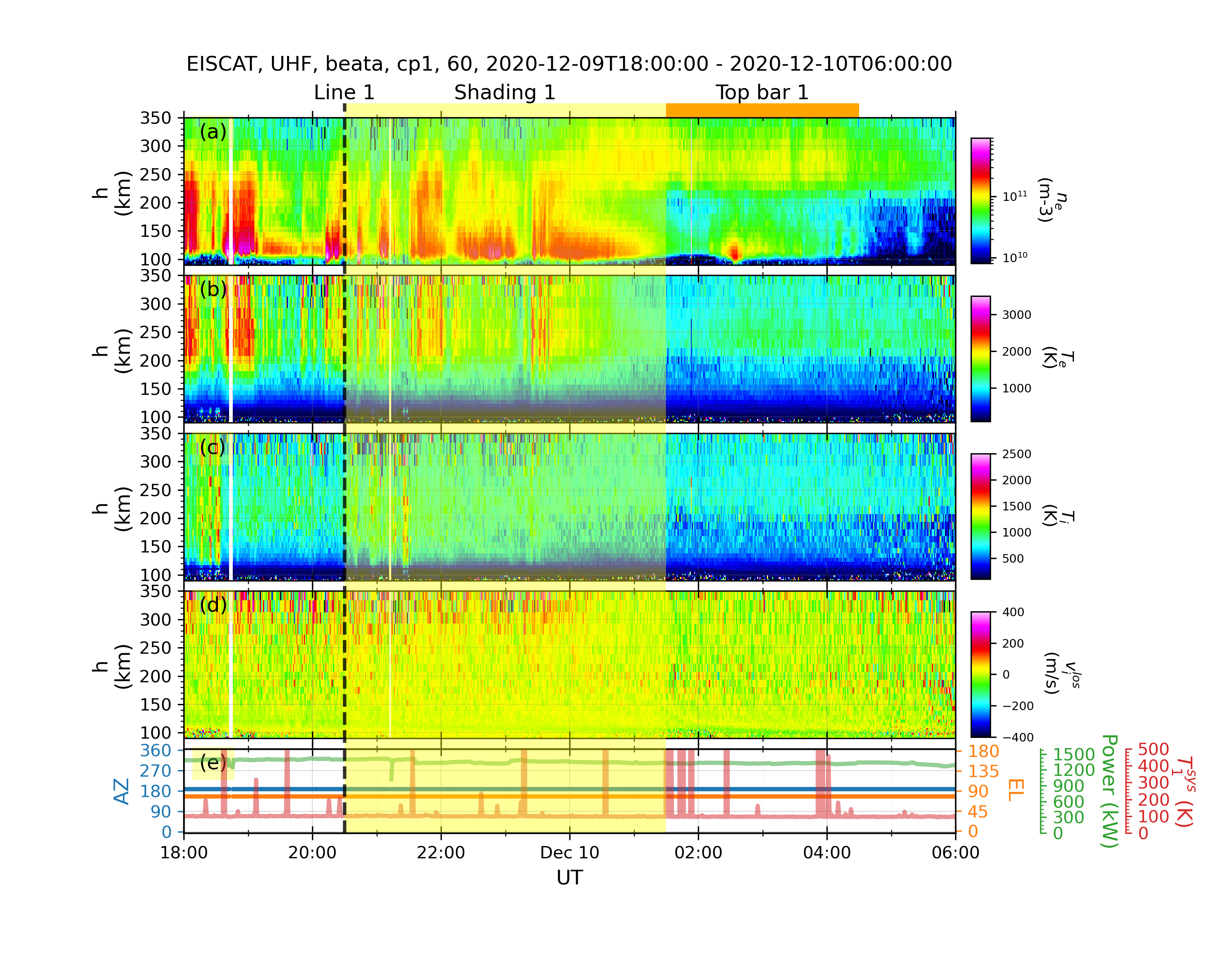
### Example 2: EISCAT quicklook plot
The EISCAT quicklook plot shows the GUISDAP analysed results in the same format as the online EISCAT quicklook plot.
The figure layout and quality are improved. In addition, several marking tools like vertical lines, shadings, top bars can be
added in the plot. See the example script and figure below:
In "example2.py"
```python
import datetime
import geospacelab.express.eiscat_dashboard as eiscat
dt_fr = datetime.datetime.strptime('20201209' + '1800', '%Y%m%d%H%M')
dt_to = datetime.datetime.strptime('20201210' + '0600', '%Y%m%d%H%M')
site = 'UHF'
antenna = 'UHF'
modulation = '60'
load_mode = 'AUTO'
dashboard = eiscat.EISCATDashboard(
dt_fr, dt_to, site=site, antenna=antenna, modulation=modulation, load_mode='AUTO'
)
dashboard.quicklook()
# dashboard.save_figure() # comment this if you need to run the following codes
# dashboard.show() # comment this if you need to run the following codes.
"""
As the dashboard class (EISCATDashboard) is a inheritance of the classes Datahub and TSDashboard.
The variables can be retrieved in the same ways as shown in Example 1.
"""
n_e = dashboard.assign_variable('n_e')
print(n_e.value)
print(n_e.error)
"""
Several marking tools (vertical lines, shadings, and top bars) can be added as the overlays
on the top of the quicklook plot.
"""
# add vertical line
dt_fr_2 = datetime.datetime.strptime('20201209' + '2030', "%Y%m%d%H%M")
dt_to_2 = datetime.datetime.strptime('20201210' + '0130', "%Y%m%d%H%M")
dashboard.add_vertical_line(dt_fr_2, bottom_extend=0, top_extend=0.02, label='Line 1', label_position='top')
# add shading
dashboard.add_shading(dt_fr_2, dt_to_2, bottom_extend=0, top_extend=0.02, label='Shading 1', label_position='top')
# add top bar
dt_fr_3 = datetime.datetime.strptime('20201210' + '0130', "%Y%m%d%H%M")
dt_to_3 = datetime.datetime.strptime('20201210' + '0430', "%Y%m%d%H%M")
dashboard.add_top_bar(dt_fr_3, dt_to_3, bottom=0., top=0.02, label='Top bar 1')
# save figure
dashboard.save_figure()
# show on screen
dashboard.show()
```
Output:
> 
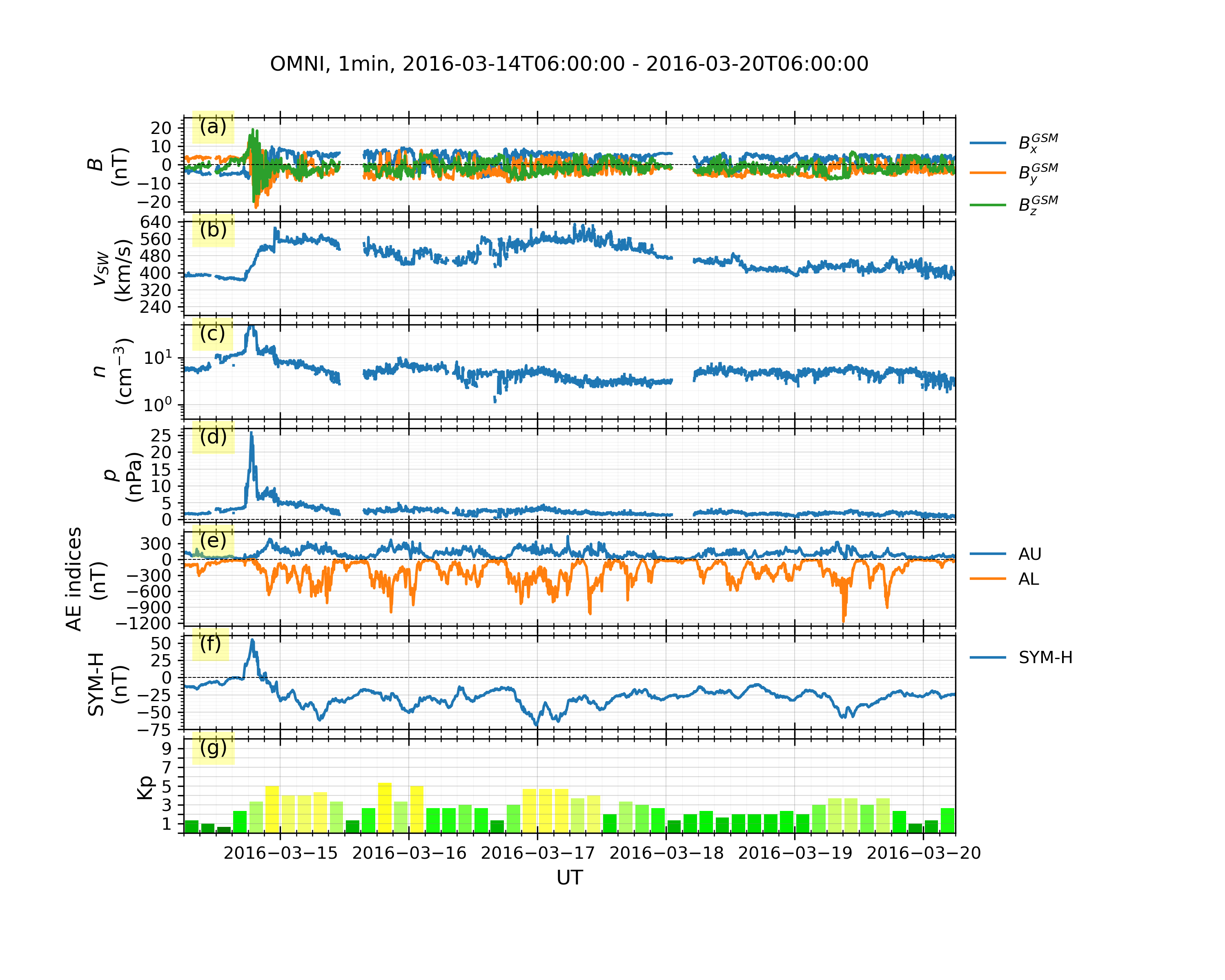
### Example 3: OMNI data and geomagnetic indices (WDC + GFZ):
In "example3.py"
```python
import datetime
import geospacelab.express.omni_dashboard as omni
dt_fr = datetime.datetime.strptime('20160314' + '0600', '%Y%m%d%H%M')
dt_to = datetime.datetime.strptime('20160320' + '0600', '%Y%m%d%H%M')
omni_type = 'OMNI2'
omni_res = '1min'
load_mode = 'AUTO'
dashboard = omni.OMNIDashboard(
dt_fr, dt_to, omni_type=omni_type, omni_res=omni_res, load_mode=load_mode
)
dashboard.quicklook()
# data can be retrieved in the same way as in Example 1:
dashboard.list_assigned_variables()
B_x_gsm = dashboard.get_variable('B_x_GSM', dataset_index=0)
# save figure
dashboard.save_figure()
# show on screen
dashboard.show()
```
Output:
> 
### Example 4: Mapping geospatial data in the polar map.
```python
import datetime
import matplotlib.pyplot as plt
import geospacelab.visualization.mpl.geomap.geodashboards as geomap
dt_fr = datetime.datetime(2015, 9, 8, 8)
dt_to = datetime.datetime(2015, 9, 8, 23, 59)
time1 = datetime.datetime(2015, 9, 8, 20, 21)
pole = 'N'
sat_id = 'f16'
band = 'LBHS'
# Create a geodashboard object
dashboard = geomap.GeoDashboard(dt_fr=dt_fr, dt_to=dt_to, figure_config={'figsize': (5, 5)})
# If the orbit_id is specified, only one file will be downloaded. This option saves the downloading time.
# dashboard.dock(datasource_contents=['jhuapl', 'dmsp', 'ssusi', 'edraur'], pole='N', sat_id='f17', orbit_id='46863')
# If not specified, the data during the whole day will be downloaded.
dashboard.dock(datasource_contents=['jhuapl', 'dmsp', 'ssusi', 'edraur'], pole=pole, sat_id=sat_id, orbit_id=None)
ds_s1 = dashboard.dock(
datasource_contents=['madrigal', 'satellites', 'dmsp', 's1'],
dt_fr=time1 - datetime.timedelta(minutes=45),
dt_to=time1 + datetime.timedelta(minutes=45),
sat_id=sat_id)
dashboard.set_layout(1, 1)
# Get the variables: LBHS emission intensiy, corresponding times and locations
lbhs = dashboard.assign_variable('GRID_AUR_' + band, dataset_index=0)
dts = dashboard.assign_variable('DATETIME', dataset_index=0).value.flatten()
mlat = dashboard.assign_variable('GRID_MLAT', dataset_index=0).value
mlon = dashboard.assign_variable('GRID_MLON', dataset_index=0).value
mlt = dashboard.assign_variable(('GRID_MLT'), dataset_index=0).value
# Search the index for the time to plot, used as an input to the following polar map
ind_t = dashboard.datasets[0].get_time_ind(ut=time1)
lbhs_ = lbhs.value[ind_t]
mlat_ = mlat[ind_t]
mlon_ = mlon[ind_t]
mlt_ = mlt[ind_t]
# Add a polar map panel to the dashboard. Currently the style is the fixed MLT at mlt_c=0. See the keywords below:
panel1 = dashboard.add_polar_map(row_ind=0, col_ind=0, style='mlt-fixed', cs='AACGM', mlt_c=0., pole=pole, ut=time1, boundary_lat=65., mirror_south=True)
# Some settings for plotting.
pcolormesh_config = lbhs.visual.plot_config.pcolormesh
# Overlay the SSUSI image in the map.
ipm = panel1.overlay_pcolormesh(data=lbhs_, coords={'lat': mlat_, 'lon': mlon_, 'mlt': mlt_}, cs='AACGM',
regridding=True, **pcolormesh_config)
# Add a color bar
panel1.add_colorbar(ipm, c_label=band + " (R)", c_scale=pcolormesh_config['c_scale'], left=1.1, bottom=0.1,
width=0.05, height=0.7)
# Overlay the gridlines
panel1.overlay_gridlines(lat_res=5, lon_label_separator=5)
# Overlay the coastlines in the AACGM coordinate
panel1.overlay_coastlines()
# Overlay cross-track velocity along satellite trajectory
sc_dt = ds_s1['SC_DATETIME'].value.flatten()
sc_lat = ds_s1['SC_GEO_LAT'].value.flatten()
sc_lon = ds_s1['SC_GEO_LON'].value.flatten()
sc_alt = ds_s1['SC_GEO_ALT'].value.flatten()
sc_coords = {'lat': sc_lat, 'lon': sc_lon, 'height': sc_alt}
v_H = ds_s1['v_i_H'].value.flatten()
panel1.overlay_cross_track_vector(vector=v_H, unit_vector=1000, alpha=0.5, color='r', sc_coords=sc_coords, sc_ut=sc_dt, cs='GEOC')
# Overlay the satellite trajectory with ticks
panel1.overlay_sc_trajectory(sc_ut=sc_dt, sc_coords=sc_coords, cs='GEOC')
# Add the title and save the figure
polestr = 'North' if pole == 'N' else 'South'
panel1.add_title(title='DMSP/SSUSI, ' + band + ', ' + sat_id.upper() + ', ' + polestr + ', ' + time1.strftime('%Y-%m-%d %H%M UT'))
plt.savefig('DMSP_SSUSI_' + time1.strftime('%Y%m%d-%H%M') + '_' + band + '_' + sat_id.upper() + '_' + pole, dpi=300)
# show the figure
plt.show()
```
Output:
> 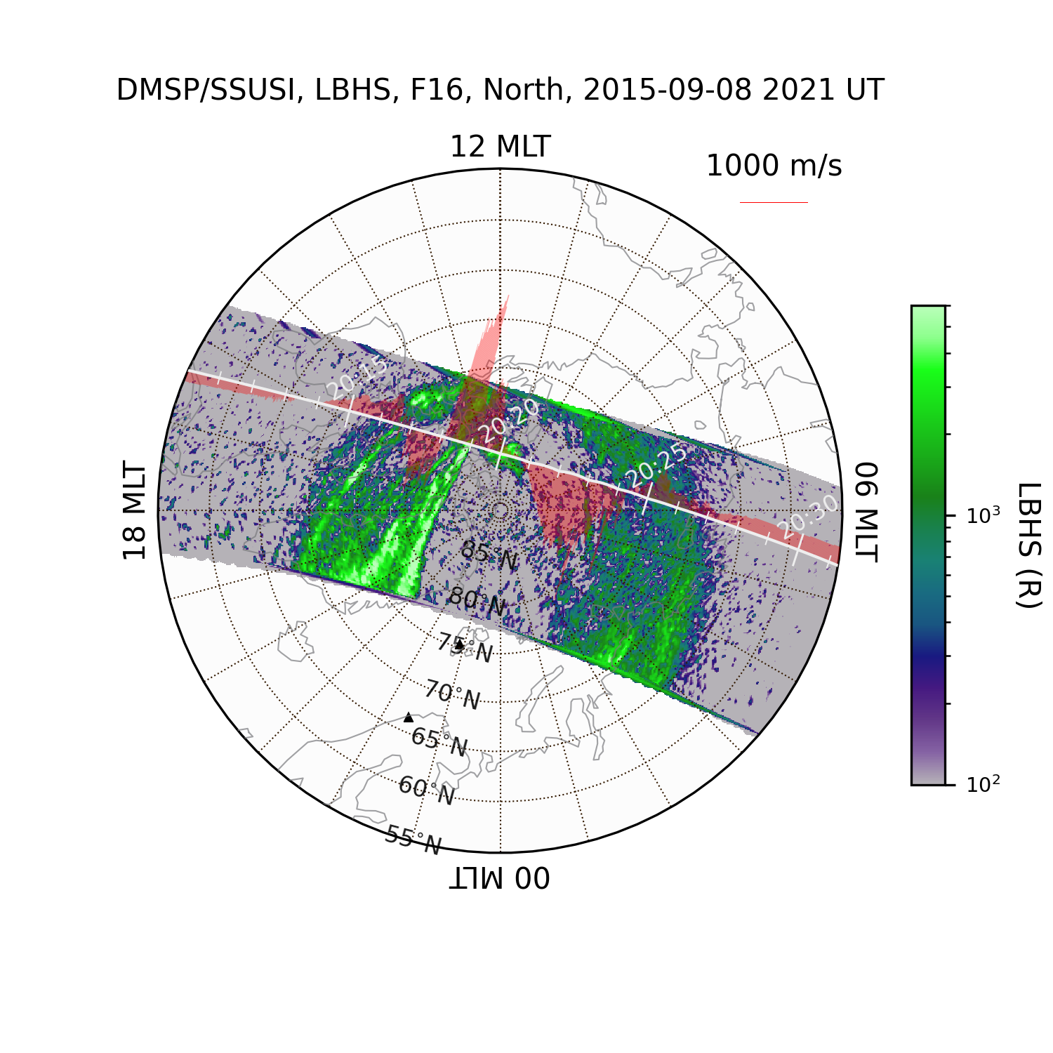
This is an example showing the HiLDA aurora in the dayside polar cap region
(see also [DMSP observations of the HiLDA aurora (Cai et al., JGR, 2021)](https://agupubs.onlinelibrary.wiley.com/doi/10.1029/2020JA028808)).
Other examples for the time-series plots and map projections can be found [here](https://github.com/JouleCai/geospacelab/tree/master/examples)
## Acknowledgements and Citation
### Acknowledgements
We acknowledge all the dependencies listed above for their contributions to implement a lot of functionality in GeospaceLAB.
### Citation
If GeospaceLAB is used for your scientific work, please mention it in the publication and cite the package:
> Cai L, Aikio A, Kullen A, Deng Y, Zhang Y, Zhang S-R, Virtanen I and Vanhamäki H (2022), GeospaceLAB: Python package
for managing and visualizing data in space physics. Front. Astron. Space Sci. 9:1023163. doi: [10.3389/fspas.2022.1023163](https://www.frontiersin.org/articles/10.3389/fspas.2022.1023163/full)
In addition, please add the following text in the "Methods" or "Acknowledgements" section:
> This research has made use of GeospaceLAB v?.?.?, an open-source Python package to manage and visualize data in space physics.
Please include the project logo (see the top) to acknowledge GeospaceLAB in posters or talks.
### Co-authorship
GeospaceLAB aims to help users to manage and visualize multiple kinds of data in space physics in a convenient way. We welcome collaboration to support your research work. If the functionality of GeospaceLAB plays a critical role in a research paper, the co-authorship is expected to be offered to one or more developers.
## Notes
- The current version is a pre-released version. Many features will be added soon.
Raw data
{
"_id": null,
"home_page": "https://github.com/JouleCai/geospacelab",
"name": "geospacelab",
"maintainer": null,
"docs_url": null,
"requires_python": ">=3.7",
"maintainer_email": null,
"keywords": "Geospace, EISCAT, DMSP, Space weather, Ionosphere, Space, Magnetosphere",
"author": "Lei Cai",
"author_email": "lei.cai@oulu.fi",
"download_url": "https://files.pythonhosted.org/packages/69/71/77886e4613c05a485d0d5568e45b2318e1bdb15a12f1a529ddf13e4104d2/geospacelab-0.8.15.tar.gz",
"platform": null,
"description": "<p align=\"center\">\n <img width=\"500\" src=\"https://github.com/JouleCai/geospacelab/blob/master/docs/images/logo_v1_landscape_accent_colors.png\">\n</p>\n\n# GeospaceLAB (geospacelab)\n[](https://opensource.org/licenses/BSD-3-Clause)\n[](https://www.python.org/) \n[](https://zenodo.org/badge/latestdoi/347315860)\n[](https://pepy.tech/project/geospacelab)\n\n[](https://pypi.python.org/pypi/geospacelab/)\n\n\nGeospaceLAB provides a framework of data access, analysis, and visualization for the researchers in space physics and space weather. The documentation can be found \non [readthedocs.io](https://geospacelab.readthedocs.io/en/latest/).\n\n## Features\n- Class-based data manager, including\n - __DataHub__: the core module (top-level class) to manage data from multiple sources,\n - __Dataset__: the middle-level class to download, load, and process data from a data source, \n - __Variable__: the base-level class to store the data array of a variable with various attributes, including its \n error, name, label, unit, group, and dependencies.\n- Extendable\n - Provide a standard procedure from downloading, loading, and post-processing the data.\n - Easy to extend for a data source which has not been supported in the package.\n - Flexible to add functions for post-processing.\n- Visualization\n - Time series plots with \n - automatically adjustable time ticks and tick labels.\n - dynamical panels (flexible to add or remove panels).\n - automatically detect the time gaps.\n - useful marking tools (vertical line crossing panels, shadings, top bars, etc, see Example 2 in\n[Usage](https://github.com/JouleCai/geospacelab#usage))\n - Map projection\n - Polar views with\n - coastlines in either GEO or AACGM (APEX) coordinate system.\n - mapping in either fixed lon/mlon mode or in fixed LST/MLT mode.\n - Support 1-D or 2-D plots with\n - satellite tracks (time ticks and labels)\n - nadir colored 1-D plots\n - gridded surface plots \n- Space coordinate system transformation\n - Unified interface for cs transformations.\n- Toolboxes for data analysis\n - Basic toolboxes for numpy array, datetime, logging, python dict, list, and class.\n\n## Built-in data sources:\n| Data Source | Variables | File Format | Downloadable | Express | Status | \n|------------------------------|------------------------------------|-----------------------|---------------|-------------------------------|--------|\n| CDAWeb/OMNI | Solar wind and IMF |*cdf* | *True* | __OMNIDashboard__ | stable |\n| Madrigal/EISCAT | Ionospheric Ne, Te, Ti, ... | *EISCAT-hdf5*, *Madrigal-hdf5* | *True* | __EISCATDashboard__ | stable |\n| Madrigal/GNSS/TECMAP | Ionospheric GPS TEC map | *hdf5* | *True* | - | beta |\n| Madrigal/DMSP/s1 | DMSP SSM, SSIES, etc | *hdf5* | *True* | __DMSPTSDashboard__ | stable |\n| Madrigal/DMSP/s4 | DMSP SSIES | *hdf5* | *True* | __DMSPTSDashboard__ | stable |\n| Madrigal/DMSP/e | DMSP SSJ | *hdf5* | *True* | __DMSPTSDashboard__ | stable |\n| Madrigal/Millstone Hill ISR+ | Millstone Hill ISR | *hdf5* | *True* | __MillstoneHillISRDashboard__ | stable |\n| Madrigal/Poker Flat ISR | Poker Flat ISR | *hdf5* | *True* | __-_ | stable |\n| JHUAPL/DMSP/SSUSI | DMSP SSUSI | *netcdf* | *True* | __DMSPSSUSIDashboard__ | stable |\n| JHUAPL/AMPERE/fitted | AMPERE FAC | *netcdf* | *False* | __AMPEREDashboard__ | stable |\n| SuperDARN/POTMAP | SuperDARN potential map | *ascii* | *False* | - | stable | \n| WDC/Dst | Dst index | *IAGA2002-ASCII* | *True* | - | stable |\n| WDC/ASYSYM | ASY/SYM indices | *IAGA2002-ASCII* | *True* | __OMNIDashboard__ | stable |\n| WDC/AE | AE indices | *IAGA2002-ASCII* | *True* | __OMNIDashboard__ | stable |\n| GFZ/Kp | Kp/Ap indices | *ASCII* | *True* | - | stable |\n| GFZ/Hpo | Hp30 or Hp60 indices | *ASCII* | *True* | - | stable |\n| GFZ/SNF107 | SN, F107 | *ASCII* | *True* | - | stable |\n| ESA/SWARM/EFI_LP_HM | SWARM Ne, Te, etc. | *netcdf* | *True* | - | stable |\n| ESA/SWARM/EFI_TCT02 | SWARM cross track vi | *netcdf* | *True* | - | stable |\n| ESA/SWARM/AOB_FAC_2F | SWARM FAC, auroral oval boundary | *netcdf* | *True* | - | beta |\n| TUDelft/SWARM/DNS_POD | Swarm $\\rho_n$ (GPS derived) | *ASCII* | *True* | - | stable |\n| TUDelft/SWARM/DNS_ACC | Swarm $\\rho_n$ (GPS+Accelerometer) | *ASCII* | *True* | - | stable |\n| TUDelft/GOCE/WIND_ACC | GOCE neutral wind | *ASCII* | *True* | - | stable |\n| TUDelft/GRACE/WIND_ACC | GRACE neutral wind | *ASCII* | *True* | - | stable |\n| TUDelft/GRACE/DNS_ACC | Grace $\\rho_n$ | *ASCII* | *True* | - | stable |\n| TUDelft/CHAMP/DNS_ACC | CHAMP $\\rho_n$ | *ASCII* | *True* | - | stable |\n | UTA/GITM/2DALL | GITM 2D output | *binary*, *IDL-sav* | *False* | - | beta |\n | UTA/GITM/3DALL | GITM 3D output | *binary*, *IDL-sav* | *False* | - | beta |\n\n\n\n## Installation\n### 1. The python distribution \"*__Anaconda__*\" is recommended:\nThe package was tested with the anaconda distribution and with **PYTHON>=3.7** under **Ubuntu 20.04** and **MacOS Big Sur**.\n\nWith Anaconda, it may be easier to install some required dependencies listed below, e.g., cartopy, using the _conda_ command.\nIt's also recommended installing the package and dependencies in a virtual environment with anaconda. \n\nAfter [installing the anaconda distribution](https://docs.anaconda.com/anaconda/install/index.html), a virtual environment can be created by the code below in the terminal:\n\n```shell\nconda create --name [YOUR_ENV_NAME] -c conda-forge python cython cartopy\n```\nThe package \"spyder\" is a widely-used python IDE. Other IDEs, like \"VS Code\" or \"Pycharm\" also work.\n\n> **_Note:_** The recommended IDE is Spyder. Sometimes, a *RuntimeError* can be raised \n> when the __aacgmv2__ package is called in **PyCharm** or **VS Code**. \n> If you meet this issue, try to compile the codes in **Spyder** several times. \n\nAfter creating the virtual environement, you need to activate the virtual environment:\n\n```shell\nconda activate [YOUR_ENV_NAME]\n```\nand then to install the package as shown below or to start the IDE **Spyder**.\n\nMore detailed information to set the anaconda environment can be found [here](https://conda.io/projects/conda/en/latest/user-guide/tasks/manage-environments.html#), \n\n### 2. Installation\n#### Quick install from the pre-built release (recommended):\n```shell\npip install geospacelab\n```\n\n#### Install from [Github](https://github.com/JouleCai/geospacelab) (not recommended):\n```shell\npip install git+https://github.com/JouleCai/geospacelab@master\n```\n\n### 2. Dependencies\nThe package dependencies need to be installed before or after the installation of the package. \nSeveral dependencies will be installed automatically with the package installation, \nincluding __toml__, __requests__, __bueatifulsoup4__, __numpy__, __scipy__, __matplotlib__, __h5py__, __netcdf4__,\n__cdflib__, __madrigalweb__, __sscws__, and __aacgmv2__.\n\nOther dependencies will be needed if you see a *__ImportError__* or *__ModuleNotFoundError__* \ndisplayed in the python console. Some frequently used modules and their installation methods are listed below:\n- [__cartopy__](https://scitools.org.uk/cartopy/docs/latest/installing.html): Map projection for geospatial data.\n - ```conda install -c conda-forge cartopy ``` \n- [__apexpy__ \\*](https://apexpy.readthedocs.io/en/latest/reference/Apex.html): Apex and Quasi-Dipole geomagnetic \ncoordinate system. \n - ```pip install apexpy ```\n- [__geopack__](https://github.com/tsssss/geopack): The geopack and Tsyganenko models in Python.\n - ```pip install geopack ```\n\n> ([\\*]()): The **_gcc_** or **_gfortran_** compilers are required before installing the package. \n> - gcc: ```conda install -c conda-forge gcc``` \n> - gfortran: ```conda install -c conda-forge gfortran ``` \n\nPlease install the packages above, if needed.\n\nNote: The package is currently pre-released. The installation methods may be changed in the future.\n\n\n### 4. First-time startup and basic configuration\nSome basic configurations will be made with the first-time import of the package. Following the messages prompted in the python console, the first configuration is to set the root directory for storing the data.\n\nWhen the modules to access the online Madrigal database is imported, it will ask for the inputs of user's full name, email, and affiliation.\n\nThe user's configuration can be found from the *__toml__* file below:\n```\n[your_home_directory]/.geospacelab/config.toml\n```\nThe user can set or change the preferences in the configuration file. For example, to change the root directory for storing the data, modify or add the lines in \"config.toml\":\n```toml\n[datahub]\ndata_root_dir = \"YOUR_ROOT_DIR\"\n```\nTo set the Madrigal cookies, change the lines:\n```toml\n[datahub.madrigal]\nuser_fullname = \"YOUR_NAME\"\nuser_email = \"YOU_EMAIL\"\nuser_affiliation = \"YOUR_AFFILIATION\"\n```\n\n### 5. Upgrade\n\nIf the package is installed from the pre-built release. Update the package via:\n```shell\npip install geospacelab --upgrade\n```\n\n### 6. Uninstallation\nUninstall the package via:\n```shell\npip uninstall geospacelab\n```\nIf you don't need the user's configuration, delete the file at **_[your_home_directory]/.geospacelab/config.toml_**\n\n## Usage\n### Example 1: Dock a sourced dataset and get variables:\nThe core of the data manager is the class Datahub. A Datahub instance will be used for docking a buit-in sourced dataset, or adding a temporary or user-defined dataset. \n\nThe \"dataset\" is a Dataset instance, which is used for loading and downloading \nthe data. \n\nBelow is an example to load the EISCAT data from the online service. The module will download EISCAT data automatically from \n[the EISCAT schedule page](https://portal.eiscat.se/schedule/) with the presetttings of loading mode \"AUTO\" and file type \"eiscat-hdf5\". \n\nExample 1:\n```python\nimport datetime\n\nfrom geospacelab.datahub import DataHub\n\n# settings\ndt_fr = datetime.datetime.strptime('20210309' + '0000', '%Y%m%d%H%M') # datetime from\ndt_to = datetime.datetime.strptime('20210309' + '2359', '%Y%m%d%H%M') # datetime to\ndatabase_name = 'madrigal' # built-in sourced database name \nfacility_name = 'eiscat' # facility name\n\nsite = 'UHF' # facility attributes required, check from the eiscat schedule page\nantenna = 'UHF'\nmodulation = 'ant'\n\n# create a datahub instance\ndh = DataHub(dt_fr, dt_to)\n# dock the first dataset (dataset index starts from 0)\nds_isr = dh.dock(datasource_contents=[database_name, 'isr', facility_name],\n site=site, antenna=antenna, modulation=modulation, data_file_type='eiscat-hdf5')\n# load data\nds_isr.load_data()\n# assign a variable from its own dataset to the datahub\nn_e = dh.assign_variable('n_e')\nT_i = dh.assign_variable('T_i')\n\n# get the variables which have been assigned in the datahub\nn_e = dh.get_variable('n_e')\nT_i = dh.get_variable('T_i')\n# if the variable is not assigned in the datahub, but exists in the its own dataset:\ncomp_O_p = dh.get_variable('comp_O_p', dataset=ds_isr) # O+ ratio\n# above line is equivalent to\ncomp_O_p = dh.datasets[0]['comp_O_p']\n\n# The variables, e.g., n_e and T_i, are the class Variable's instances, \n# which stores the variable values, errors, and many other attributes, e.g., name, label, unit, depends, ....\n# To get the value of the variable, use variable_isntance.value, e.g.,\nprint(n_e.value) # return the variable's value, type: numpy.ndarray, axis 0 is always along the time, check n_e.depends.items{}\nprint(n_e.error)\n\n```\n\n### Example 2: EISCAT quicklook plot\nThe EISCAT quicklook plot shows the GUISDAP analysed results in the same format as the online EISCAT quicklook plot.\nThe figure layout and quality are improved. In addition, several marking tools like vertical lines, shadings, top bars can be \nadded in the plot. See the example script and figure below:\n\nIn \"example2.py\"\n```python\nimport datetime\nimport geospacelab.express.eiscat_dashboard as eiscat\n\ndt_fr = datetime.datetime.strptime('20201209' + '1800', '%Y%m%d%H%M')\ndt_to = datetime.datetime.strptime('20201210' + '0600', '%Y%m%d%H%M')\n\nsite = 'UHF'\nantenna = 'UHF'\nmodulation = '60'\nload_mode = 'AUTO'\ndashboard = eiscat.EISCATDashboard(\n dt_fr, dt_to, site=site, antenna=antenna, modulation=modulation, load_mode='AUTO'\n)\ndashboard.quicklook()\n\n# dashboard.save_figure() # comment this if you need to run the following codes\n# dashboard.show() # comment this if you need to run the following codes.\n\n\"\"\"\nAs the dashboard class (EISCATDashboard) is a inheritance of the classes Datahub and TSDashboard.\nThe variables can be retrieved in the same ways as shown in Example 1. \n\"\"\"\nn_e = dashboard.assign_variable('n_e')\nprint(n_e.value)\nprint(n_e.error)\n\n\"\"\"\nSeveral marking tools (vertical lines, shadings, and top bars) can be added as the overlays \non the top of the quicklook plot.\n\"\"\"\n# add vertical line\ndt_fr_2 = datetime.datetime.strptime('20201209' + '2030', \"%Y%m%d%H%M\")\ndt_to_2 = datetime.datetime.strptime('20201210' + '0130', \"%Y%m%d%H%M\")\ndashboard.add_vertical_line(dt_fr_2, bottom_extend=0, top_extend=0.02, label='Line 1', label_position='top')\n# add shading\ndashboard.add_shading(dt_fr_2, dt_to_2, bottom_extend=0, top_extend=0.02, label='Shading 1', label_position='top')\n# add top bar\ndt_fr_3 = datetime.datetime.strptime('20201210' + '0130', \"%Y%m%d%H%M\")\ndt_to_3 = datetime.datetime.strptime('20201210' + '0430', \"%Y%m%d%H%M\")\ndashboard.add_top_bar(dt_fr_3, dt_to_3, bottom=0., top=0.02, label='Top bar 1')\n\n# save figure\ndashboard.save_figure()\n# show on screen\ndashboard.show()\n```\nOutput:\n> \n\n### Example 3: OMNI data and geomagnetic indices (WDC + GFZ):\n\nIn \"example3.py\"\n\n```python\nimport datetime\nimport geospacelab.express.omni_dashboard as omni\n\ndt_fr = datetime.datetime.strptime('20160314' + '0600', '%Y%m%d%H%M')\ndt_to = datetime.datetime.strptime('20160320' + '0600', '%Y%m%d%H%M')\n\nomni_type = 'OMNI2'\nomni_res = '1min'\nload_mode = 'AUTO'\ndashboard = omni.OMNIDashboard(\n dt_fr, dt_to, omni_type=omni_type, omni_res=omni_res, load_mode=load_mode\n)\ndashboard.quicklook()\n\n# data can be retrieved in the same way as in Example 1:\ndashboard.list_assigned_variables()\nB_x_gsm = dashboard.get_variable('B_x_GSM', dataset_index=0)\n# save figure\ndashboard.save_figure()\n# show on screen\ndashboard.show()\n```\nOutput:\n> \n\n### Example 4: Mapping geospatial data in the polar map.\n```python\nimport datetime\nimport matplotlib.pyplot as plt\n\nimport geospacelab.visualization.mpl.geomap.geodashboards as geomap\n\ndt_fr = datetime.datetime(2015, 9, 8, 8)\ndt_to = datetime.datetime(2015, 9, 8, 23, 59)\ntime1 = datetime.datetime(2015, 9, 8, 20, 21)\npole = 'N'\nsat_id = 'f16'\nband = 'LBHS'\n\n# Create a geodashboard object\ndashboard = geomap.GeoDashboard(dt_fr=dt_fr, dt_to=dt_to, figure_config={'figsize': (5, 5)})\n\n# If the orbit_id is specified, only one file will be downloaded. This option saves the downloading time.\n# dashboard.dock(datasource_contents=['jhuapl', 'dmsp', 'ssusi', 'edraur'], pole='N', sat_id='f17', orbit_id='46863')\n# If not specified, the data during the whole day will be downloaded.\ndashboard.dock(datasource_contents=['jhuapl', 'dmsp', 'ssusi', 'edraur'], pole=pole, sat_id=sat_id, orbit_id=None)\nds_s1 = dashboard.dock(\n datasource_contents=['madrigal', 'satellites', 'dmsp', 's1'],\n dt_fr=time1 - datetime.timedelta(minutes=45),\n dt_to=time1 + datetime.timedelta(minutes=45),\n sat_id=sat_id)\n\ndashboard.set_layout(1, 1)\n\n# Get the variables: LBHS emission intensiy, corresponding times and locations\nlbhs = dashboard.assign_variable('GRID_AUR_' + band, dataset_index=0)\ndts = dashboard.assign_variable('DATETIME', dataset_index=0).value.flatten()\nmlat = dashboard.assign_variable('GRID_MLAT', dataset_index=0).value\nmlon = dashboard.assign_variable('GRID_MLON', dataset_index=0).value\nmlt = dashboard.assign_variable(('GRID_MLT'), dataset_index=0).value\n\n# Search the index for the time to plot, used as an input to the following polar map\nind_t = dashboard.datasets[0].get_time_ind(ut=time1)\nlbhs_ = lbhs.value[ind_t]\nmlat_ = mlat[ind_t]\nmlon_ = mlon[ind_t]\nmlt_ = mlt[ind_t]\n# Add a polar map panel to the dashboard. Currently the style is the fixed MLT at mlt_c=0. See the keywords below:\npanel1 = dashboard.add_polar_map(row_ind=0, col_ind=0, style='mlt-fixed', cs='AACGM', mlt_c=0., pole=pole, ut=time1, boundary_lat=65., mirror_south=True)\n\n# Some settings for plotting.\npcolormesh_config = lbhs.visual.plot_config.pcolormesh\n# Overlay the SSUSI image in the map.\nipm = panel1.overlay_pcolormesh(data=lbhs_, coords={'lat': mlat_, 'lon': mlon_, 'mlt': mlt_}, cs='AACGM',\n regridding=True, **pcolormesh_config)\n# Add a color bar\npanel1.add_colorbar(ipm, c_label=band + \" (R)\", c_scale=pcolormesh_config['c_scale'], left=1.1, bottom=0.1,\n width=0.05, height=0.7)\n\n# Overlay the gridlines\npanel1.overlay_gridlines(lat_res=5, lon_label_separator=5)\n\n# Overlay the coastlines in the AACGM coordinate\npanel1.overlay_coastlines()\n\n# Overlay cross-track velocity along satellite trajectory\nsc_dt = ds_s1['SC_DATETIME'].value.flatten()\nsc_lat = ds_s1['SC_GEO_LAT'].value.flatten()\nsc_lon = ds_s1['SC_GEO_LON'].value.flatten()\nsc_alt = ds_s1['SC_GEO_ALT'].value.flatten()\nsc_coords = {'lat': sc_lat, 'lon': sc_lon, 'height': sc_alt}\n\nv_H = ds_s1['v_i_H'].value.flatten()\npanel1.overlay_cross_track_vector(vector=v_H, unit_vector=1000, alpha=0.5, color='r', sc_coords=sc_coords, sc_ut=sc_dt, cs='GEOC')\n# Overlay the satellite trajectory with ticks\npanel1.overlay_sc_trajectory(sc_ut=sc_dt, sc_coords=sc_coords, cs='GEOC')\n\n# Add the title and save the figure\npolestr = 'North' if pole == 'N' else 'South'\npanel1.add_title(title='DMSP/SSUSI, ' + band + ', ' + sat_id.upper() + ', ' + polestr + ', ' + time1.strftime('%Y-%m-%d %H%M UT'))\nplt.savefig('DMSP_SSUSI_' + time1.strftime('%Y%m%d-%H%M') + '_' + band + '_' + sat_id.upper() + '_' + pole, dpi=300)\n\n# show the figure\nplt.show()\n```\nOutput:\n> \n\nThis is an example showing the HiLDA aurora in the dayside polar cap region \n(see also [DMSP observations of the HiLDA aurora (Cai et al., JGR, 2021)](https://agupubs.onlinelibrary.wiley.com/doi/10.1029/2020JA028808)).\n\nOther examples for the time-series plots and map projections can be found [here](https://github.com/JouleCai/geospacelab/tree/master/examples)\n\n## Acknowledgements and Citation\n### Acknowledgements\nWe acknowledge all the dependencies listed above for their contributions to implement a lot of functionality in GeospaceLAB.\n\n### Citation\nIf GeospaceLAB is used for your scientific work, please mention it in the publication and cite the package:\n> Cai L, Aikio A, Kullen A, Deng Y, Zhang Y, Zhang S-R, Virtanen I and Vanham\u00e4ki H (2022), GeospaceLAB: Python package \nfor managing and visualizing data in space physics. Front. Astron. Space Sci. 9:1023163. doi: [10.3389/fspas.2022.1023163](https://www.frontiersin.org/articles/10.3389/fspas.2022.1023163/full)\n\nIn addition, please add the following text in the \"Methods\" or \"Acknowledgements\" section: \n> This research has made use of GeospaceLAB v?.?.?, an open-source Python package to manage and visualize data in space physics. \n\nPlease include the project logo (see the top) to acknowledge GeospaceLAB in posters or talks. \n\n### Co-authorship\nGeospaceLAB aims to help users to manage and visualize multiple kinds of data in space physics in a convenient way. We welcome collaboration to support your research work. If the functionality of GeospaceLAB plays a critical role in a research paper, the co-authorship is expected to be offered to one or more developers.\n\n\n## Notes\n- The current version is a pre-released version. Many features will be added soon.\n\n\n",
"bugtrack_url": null,
"license": "BSD 3-Clause License",
"summary": "Collect, manage, and visualize geospace data.",
"version": "0.8.15",
"project_urls": {
"Homepage": "https://github.com/JouleCai/geospacelab"
},
"split_keywords": [
"geospace",
" eiscat",
" dmsp",
" space weather",
" ionosphere",
" space",
" magnetosphere"
],
"urls": [
{
"comment_text": "",
"digests": {
"blake2b_256": "697177886e4613c05a485d0d5568e45b2318e1bdb15a12f1a529ddf13e4104d2",
"md5": "8b0f1cb4bd0f59040a0bf064d5b1da41",
"sha256": "63acbad2722043557613c22f3f1cf13ba0cf2a2b256cc8af60ee311452b4a92f"
},
"downloads": -1,
"filename": "geospacelab-0.8.15.tar.gz",
"has_sig": false,
"md5_digest": "8b0f1cb4bd0f59040a0bf064d5b1da41",
"packagetype": "sdist",
"python_version": "source",
"requires_python": ">=3.7",
"size": 401798,
"upload_time": "2025-01-29T13:10:55",
"upload_time_iso_8601": "2025-01-29T13:10:55.005419Z",
"url": "https://files.pythonhosted.org/packages/69/71/77886e4613c05a485d0d5568e45b2318e1bdb15a12f1a529ddf13e4104d2/geospacelab-0.8.15.tar.gz",
"yanked": false,
"yanked_reason": null
}
],
"upload_time": "2025-01-29 13:10:55",
"github": true,
"gitlab": false,
"bitbucket": false,
"codeberg": false,
"github_user": "JouleCai",
"github_project": "geospacelab",
"travis_ci": false,
"coveralls": false,
"github_actions": false,
"lcname": "geospacelab"
}

