# kalepy: Kernel Density Estimation and Sampling
[](https://github.com/lzkelley/kalepy/actions/workflows/main.yml)
[](https://codecov.io/gh/lzkelley/kalepy)
[](https://kalepy.readthedocs.io/en/latest/?badge=latest)
[](https://doi.org/10.21105/joss.02784)
[](https://zenodo.org/badge/latestdoi/187267055)

This package performs KDE operations on multidimensional data to: **1) calculate estimated PDFs** (probability distribution functions), and **2) resample new data** from those PDFs.
## Documentation
A number of examples (also used for continuous integration testing) are included in [the package notebooks](https://github.com/lzkelley/kalepy/tree/master/notebooks). Some background information and references are included in [the JOSS paper](https://joss.theoj.org/papers/10.21105/joss.02784).
Full documentation is available on [kalepy.readthedocs.io](https://kalepy.readthedocs.io/en/latest/).
## README Contents
- [Installation](#Installation)
- Quickstart
- [Basic Usage](#Basic-Usage)
- [Fancy Usage](#Fancy-Usage)
- [Development & Contributions](#Development-&-Contributions)
- [Attribution (citation)](#Attribution)
## Installation
#### from pypi (i.e. via pip)
```bash
pip install kalepy
```
#### from source (e.g. for development)
```bash
git clone https://github.com/lzkelley/kalepy.git
pip install -e kalepy/
```
In this case the package can easily be updated by changing into the source directory, pulling, and rebuilding:
```bash
cd kalepy
git pull
pip install -e .
# Optional: run unit tests (using the `pytest` package)
pytest
```
# Basic Usage
```python
import numpy as np
import matplotlib.pyplot as plt
import matplotlib as mpl
import kalepy as kale
from kalepy.plot import nbshow
```
Generate some random data, and its corresponding distribution function
```python
NUM = int(1e4)
np.random.seed(12345)
# Combine data from two different PDFs
_d1 = np.random.normal(4.0, 1.0, NUM)
_d2 = np.random.lognormal(0, 0.5, size=NUM)
data = np.concatenate([_d1, _d2])
# Calculate the "true" distribution
xx = np.linspace(0.0, 7.0, 100)[1:]
yy = 0.5*np.exp(-(xx - 4.0)**2/2) / np.sqrt(2*np.pi)
yy += 0.5 * np.exp(-np.log(xx)**2/(2*0.5**2)) / (0.5*xx*np.sqrt(2*np.pi))
```
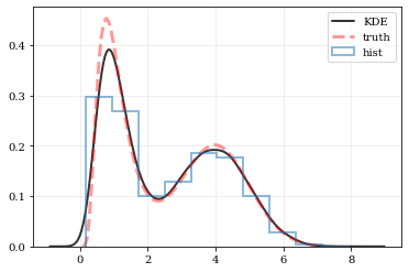
### Plotting Smooth Distributions
```python
# Reconstruct the probability-density based on the given data points.
points, density = kale.density(data, probability=True)
# Plot the PDF
plt.plot(points, density, 'k-', lw=2.0, alpha=0.8, label='KDE')
# Plot the "true" PDF
plt.plot(xx, yy, 'r--', alpha=0.4, lw=3.0, label='truth')
# Plot the standard, histogram density estimate
plt.hist(data, density=True, histtype='step', lw=2.0, alpha=0.5, label='hist')
plt.legend()
nbshow()
```
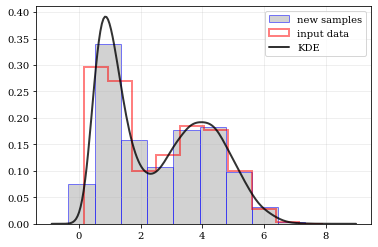
### resampling: constructing statistically similar values
Draw a new sample of data-points from the KDE PDF
```python
# Draw new samples from the KDE reconstructed PDF
samples = kale.resample(data)
# Plot new samples
plt.hist(samples, density=True, label='new samples', alpha=0.5, color='0.65', edgecolor='b')
# Plot the old samples
plt.hist(data, density=True, histtype='step', lw=2.0, alpha=0.5, color='r', label='input data')
# Plot the KDE reconstructed PDF
plt.plot(points, density, 'k-', lw=2.0, alpha=0.8, label='KDE')
plt.legend()
nbshow()
```
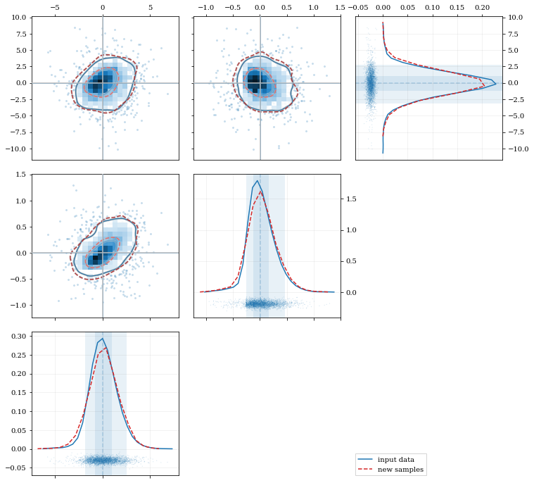
### Multivariate Distributions
```python
reload(kale.plot)
# Load some random-ish three-dimensional data
np.random.seed(9485)
data = kale.utils._random_data_3d_02(num=3e3)
# Construct a KDE
kde = kale.KDE(data)
# Construct new data by resampling from the KDE
resamp = kde.resample(size=1e3)
# Plot the data and distributions using the builtin `kalepy.corner` plot
corner, h1 = kale.corner(kde, quantiles=[0.5, 0.9])
h2 = corner.clean(resamp, quantiles=[0.5, 0.9], dist2d=dict(median=False), ls='--')
corner.legend([h1, h2], ['input data', 'new samples'])
nbshow()
```
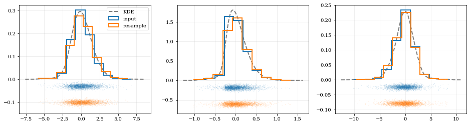
```python
# Resample the data (default output is the same size as the input data)
samples = kde.resample()
# ---- Plot the input data compared to the resampled data ----
fig, axes = plt.subplots(figsize=[16, 4], ncols=kde.ndim)
for ii, ax in enumerate(axes):
# Calculate and plot PDF for `ii`th parameter (i.e. data dimension `ii`)
xx, yy = kde.density(params=ii, probability=True)
ax.plot(xx, yy, 'k--', label='KDE', lw=2.0, alpha=0.5)
# Draw histograms of original and newly resampled datasets
*_, h1 = ax.hist(data[ii], histtype='step', density=True, lw=2.0, label='input')
*_, h2 = ax.hist(samples[ii], histtype='step', density=True, lw=2.0, label='resample')
# Add 'kalepy.carpet' plots showing the data points themselves
kale.carpet(data[ii], ax=ax, color=h1[0].get_facecolor())
kale.carpet(samples[ii], ax=ax, color=h2[0].get_facecolor(), shift=ax.get_ylim()[0])
axes[0].legend()
nbshow()
```
# Fancy Usage
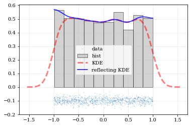
### Reflecting Boundaries
What if the distributions you're trying to capture have edges in them, like in a uniform distribution between two bounds? Here, the KDE chooses 'reflection' locations based on the extrema of the given data.
```python
# Uniform data (edges at -1 and +1)
NDATA = 1e3
np.random.seed(54321)
data = np.random.uniform(-1.0, 1.0, int(NDATA))
# Create a 'carpet' plot of the data
kale.carpet(data, label='data')
# Histogram the data
plt.hist(data, density=True, alpha=0.5, label='hist', color='0.65', edgecolor='k')
# ---- Standard KDE will undershoot just-inside the edges and overshoot outside edges
points, pdf_basic = kale.density(data, probability=True)
plt.plot(points, pdf_basic, 'r--', lw=3.0, alpha=0.5, label='KDE')
# ---- Reflecting KDE keeps probability within the given bounds
# setting `reflect=True` lets the KDE guess the edge locations based on the data extrema
points, pdf_reflect = kale.density(data, reflect=True, probability=True)
plt.plot(points, pdf_reflect, 'b-', lw=2.0, alpha=0.75, label='reflecting KDE')
plt.legend()
nbshow()
```
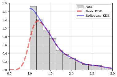
Explicit reflection locations can also be provided (in any number of dimensions).
```python
# Construct random data, add an artificial 'edge'
np.random.seed(5142)
edge = 1.0
data = np.random.lognormal(sigma=0.5, size=int(3e3))
data = data[data >= edge]
# Histogram the data, use fixed bin-positions
edges = np.linspace(edge, 4, 20)
plt.hist(data, bins=edges, density=True, alpha=0.5, label='data', color='0.65', edgecolor='k')
# Standard KDE with over & under estimates
points, pdf_basic = kale.density(data, probability=True)
plt.plot(points, pdf_basic, 'r--', lw=4.0, alpha=0.5, label='Basic KDE')
# Reflecting KDE setting the lower-boundary to the known value
# There is no upper-boundary when `None` is given.
points, pdf_basic = kale.density(data, reflect=[edge, None], probability=True)
plt.plot(points, pdf_basic, 'b-', lw=3.0, alpha=0.5, label='Reflecting KDE')
plt.gca().set_xlim(edge - 0.5, 3)
plt.legend()
nbshow()
```
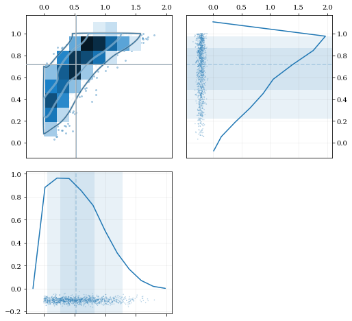
### Multivariate Reflection
```python
# Load a predefined dataset that has boundaries at:
# x: 0.0 on the low-end
# y: 1.0 on the high-end
data = kale.utils._random_data_2d_03()
# Construct a KDE with the given reflection boundaries given explicitly
kde = kale.KDE(data, reflect=[[0, None], [None, 1]])
# Plot using default settings
kale.corner(kde)
nbshow()
```
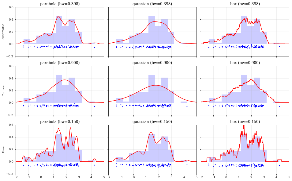
### Specifying Bandwidths and Kernel Functions
```python
# Load predefined 'random' data
data = kale.utils._random_data_1d_02(num=100)
# Choose a uniform x-spacing for drawing PDFs
xx = np.linspace(-2, 8, 1000)
# ------ Choose the kernel-functions and bandwidths to test ------- #
kernels = ['parabola', 'gaussian', 'box'] #
bandwidths = [None, 0.9, 0.15] # `None` means let kalepy choose #
# ----------------------------------------------------------------- #
ylabels = ['Automatic', 'Course', 'Fine']
fig, axes = plt.subplots(figsize=[16, 10], ncols=len(kernels), nrows=len(bandwidths), sharex=True, sharey=True)
plt.subplots_adjust(hspace=0.2, wspace=0.05)
for (ii, jj), ax in np.ndenumerate(axes):
# ---- Construct KDE using particular kernel-function and bandwidth ---- #
kern = kernels[jj] #
bw = bandwidths[ii] #
kde = kale.KDE(data, kernel=kern, bandwidth=bw) #
# ---------------------------------------------------------------------- #
# If bandwidth was set to `None`, then the KDE will choose the 'optimal' value
if bw is None:
bw = kde.bandwidth[0, 0]
ax.set_title('{} (bw={:.3f})'.format(kern, bw))
if jj == 0:
ax.set_ylabel(ylabels[ii])
# plot the KDE
ax.plot(*kde.pdf(points=xx), color='r')
# plot histogram of the data (same for all panels)
ax.hist(data, bins='auto', color='b', alpha=0.2, density=True)
# plot carpet of the data (same for all panels)
kale.carpet(data, ax=ax, color='b')
ax.set(xlim=[-2, 5], ylim=[-0.2, 0.6])
nbshow()
```
## Resampling
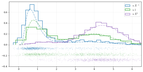
### Using different data `weights`
```python
# Load some random data (and the 'true' PDF, for comparison)
data, truth = kale.utils._random_data_1d_01()
# ---- Resample the same data, using different weightings ---- #
resamp_uni = kale.resample(data, size=1000) #
resamp_sqr = kale.resample(data, weights=data**2, size=1000) #
resamp_inv = kale.resample(data, weights=data**-1, size=1000) #
# ------------------------------------------------------------ #
# ---- Plot different distributions ----
# Setup plotting parameters
kw = dict(density=True, histtype='step', lw=2.0, alpha=0.75, bins='auto')
xx, yy = truth
samples = [resamp_inv, resamp_uni, resamp_sqr]
yvals = [yy/xx, yy, yy*xx**2/10]
labels = [r'$\propto X^{-1}$', r'$\propto 1$', r'$\propto X^2$']
plt.figure(figsize=[10, 5])
for ii, (res, yy, lab) in enumerate(zip(samples, yvals, labels)):
hh, = plt.plot(xx, yy, ls='--', alpha=0.5, lw=2.0)
col = hh.get_color()
kale.carpet(res, color=col, shift=-0.1*ii)
plt.hist(res, color=col, label=lab, **kw)
plt.gca().set(xlim=[-0.5, 6.5])
# Add legend
plt.legend()
# display the figure if this is a notebook
nbshow()
```
### Resampling while 'keeping' certain parameters/dimensions
```python
# Construct covariant 2D dataset where the 0th parameter takes on discrete values
xx = np.random.randint(2, 7, 1000)
yy = np.random.normal(4, 2, xx.size) + xx**(3/2)
data = [xx, yy]
# 2D plotting settings: disable the 2D histogram & disable masking of dense scatter-points
dist2d = dict(hist=False, mask_dense=False)
# Draw a corner plot
kale.corner(data, dist2d=dist2d)
nbshow()
```
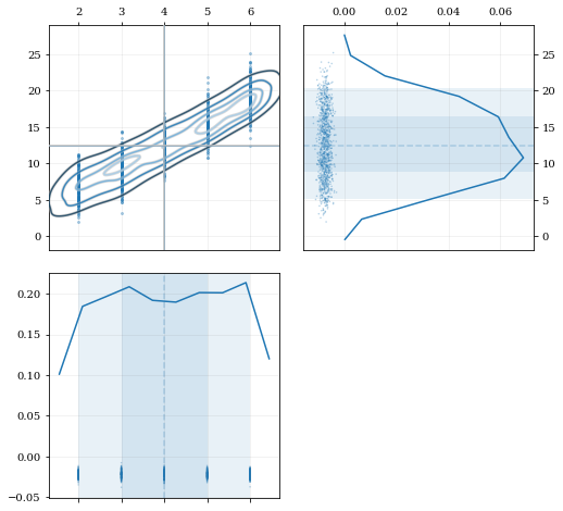
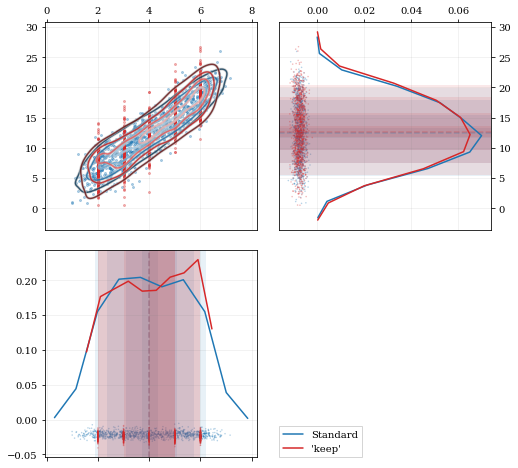
A standard KDE resampling will smooth out the discrete variables, creating a smooth(er) distribution. Using the `keep` parameter, we can choose to resample from the actual data values of that parameter instead of resampling with 'smoothing' based on the KDE.
```python
kde = kale.KDE(data)
# ---- Resample the data both normally, and 'keep'ing the 0th parameter values ---- #
resamp_stnd = kde.resample() #
resamp_keep = kde.resample(keep=0) #
# --------------------------------------------------------------------------------- #
corner = kale.Corner(2)
dist2d['median'] = False # disable median 'cross-hairs'
h1 = corner.plot(resamp_stnd, dist2d=dist2d)
h2 = corner.plot(resamp_keep, dist2d=dist2d)
corner.legend([h1, h2], ['Standard', "'keep'"])
nbshow()
```
## Development & Contributions
Please visit the `github page <https://github.com/lzkelley/kalepy>`_ for issues or bug reports. Contributions and feedback are very welcome.
Contributors:
* Luke Zoltan Kelley (@lzkelley)
* Zachary Hafen (@zhafen)
JOSS Paper:
* Kexin Rong (@kexinrong)
* Arfon Smith (@arfon)
* Will Handley (@williamjameshandley)
## Attribution
A JOSS paper has been submitted. If you have found this package useful in your research, please add a reference to the code paper:
.. code-block:: tex
@article{kalepy,
author = {Luke Zoltan Kelley},
title = {kalepy: a python package for kernel density estimation and sampling},
journal = {The Journal of Open Source Software},
publisher = {The Open Journal},
}
Raw data
{
"_id": null,
"home_page": "https://github.com/lzkelley/kalepy/",
"name": "kalepy",
"maintainer": "",
"docs_url": null,
"requires_python": ">=3.7",
"maintainer_email": "",
"keywords": "utilities,physics,astronomy,cosmology,astrophysics,statistics,kernel density estimation,kernel density estimate",
"author": "Luke Zoltan Kelley",
"author_email": "lzkelley@northwestern.edu",
"download_url": "https://files.pythonhosted.org/packages/ec/8a/dcddf5f8c8d438199482b682916fef57b207cf20c5660e1474b305b2553e/kalepy-1.4.2.tar.gz",
"platform": null,
"description": "# kalepy: Kernel Density Estimation and Sampling\n\n[](https://github.com/lzkelley/kalepy/actions/workflows/main.yml)\n[](https://codecov.io/gh/lzkelley/kalepy)\n[](https://kalepy.readthedocs.io/en/latest/?badge=latest)\n[](https://doi.org/10.21105/joss.02784)\n[](https://zenodo.org/badge/latestdoi/187267055)\n\n\n\nThis package performs KDE operations on multidimensional data to: **1) calculate estimated PDFs** (probability distribution functions), and **2) resample new data** from those PDFs.\n\n## Documentation\n\nA number of examples (also used for continuous integration testing) are included in [the package notebooks](https://github.com/lzkelley/kalepy/tree/master/notebooks). Some background information and references are included in [the JOSS paper](https://joss.theoj.org/papers/10.21105/joss.02784).\n\nFull documentation is available on [kalepy.readthedocs.io](https://kalepy.readthedocs.io/en/latest/).\n\n## README Contents\n\n- [Installation](#Installation)\n- Quickstart\n - [Basic Usage](#Basic-Usage)\n - [Fancy Usage](#Fancy-Usage)\n- [Development & Contributions](#Development-&-Contributions)\n- [Attribution (citation)](#Attribution)\n\n\n## Installation\n\n#### from pypi (i.e. via pip)\n\n```bash\npip install kalepy\n```\n\n#### from source (e.g. for development)\n\n```bash\ngit clone https://github.com/lzkelley/kalepy.git\npip install -e kalepy/\n```\n\nIn this case the package can easily be updated by changing into the source directory, pulling, and rebuilding:\n\n```bash\ncd kalepy\ngit pull\npip install -e .\n# Optional: run unit tests (using the `pytest` package)\npytest\n```\n\n\n# Basic Usage\n\n\n```python\nimport numpy as np\nimport matplotlib.pyplot as plt\nimport matplotlib as mpl\n\nimport kalepy as kale\n\nfrom kalepy.plot import nbshow\n```\n\nGenerate some random data, and its corresponding distribution function\n\n\n```python\nNUM = int(1e4)\nnp.random.seed(12345)\n# Combine data from two different PDFs\n_d1 = np.random.normal(4.0, 1.0, NUM)\n_d2 = np.random.lognormal(0, 0.5, size=NUM)\ndata = np.concatenate([_d1, _d2])\n\n# Calculate the \"true\" distribution\nxx = np.linspace(0.0, 7.0, 100)[1:]\nyy = 0.5*np.exp(-(xx - 4.0)**2/2) / np.sqrt(2*np.pi)\nyy += 0.5 * np.exp(-np.log(xx)**2/(2*0.5**2)) / (0.5*xx*np.sqrt(2*np.pi))\n```\n\n### Plotting Smooth Distributions\n\n\n```python\n# Reconstruct the probability-density based on the given data points.\npoints, density = kale.density(data, probability=True)\n\n# Plot the PDF\nplt.plot(points, density, 'k-', lw=2.0, alpha=0.8, label='KDE')\n\n# Plot the \"true\" PDF\nplt.plot(xx, yy, 'r--', alpha=0.4, lw=3.0, label='truth')\n\n# Plot the standard, histogram density estimate\nplt.hist(data, density=True, histtype='step', lw=2.0, alpha=0.5, label='hist')\n\nplt.legend()\nnbshow()\n```\n\n\n \n\n \n\n\n### resampling: constructing statistically similar values\n\nDraw a new sample of data-points from the KDE PDF\n\n\n```python\n# Draw new samples from the KDE reconstructed PDF\nsamples = kale.resample(data)\n\n# Plot new samples\nplt.hist(samples, density=True, label='new samples', alpha=0.5, color='0.65', edgecolor='b')\n# Plot the old samples\nplt.hist(data, density=True, histtype='step', lw=2.0, alpha=0.5, color='r', label='input data')\n\n# Plot the KDE reconstructed PDF\nplt.plot(points, density, 'k-', lw=2.0, alpha=0.8, label='KDE')\n\nplt.legend()\nnbshow()\n```\n\n\n \n\n \n\n\n### Multivariate Distributions\n\n\n```python\nreload(kale.plot)\n\n# Load some random-ish three-dimensional data\nnp.random.seed(9485)\ndata = kale.utils._random_data_3d_02(num=3e3)\n\n# Construct a KDE\nkde = kale.KDE(data)\n\n# Construct new data by resampling from the KDE\nresamp = kde.resample(size=1e3)\n\n# Plot the data and distributions using the builtin `kalepy.corner` plot\ncorner, h1 = kale.corner(kde, quantiles=[0.5, 0.9])\nh2 = corner.clean(resamp, quantiles=[0.5, 0.9], dist2d=dict(median=False), ls='--')\n\ncorner.legend([h1, h2], ['input data', 'new samples'])\n\nnbshow()\n```\n\n\n \n\n \n\n\n\n```python\n# Resample the data (default output is the same size as the input data)\nsamples = kde.resample()\n\n\n# ---- Plot the input data compared to the resampled data ----\n\nfig, axes = plt.subplots(figsize=[16, 4], ncols=kde.ndim)\n\nfor ii, ax in enumerate(axes):\n # Calculate and plot PDF for `ii`th parameter (i.e. data dimension `ii`)\n xx, yy = kde.density(params=ii, probability=True)\n ax.plot(xx, yy, 'k--', label='KDE', lw=2.0, alpha=0.5)\n # Draw histograms of original and newly resampled datasets\n *_, h1 = ax.hist(data[ii], histtype='step', density=True, lw=2.0, label='input')\n *_, h2 = ax.hist(samples[ii], histtype='step', density=True, lw=2.0, label='resample')\n # Add 'kalepy.carpet' plots showing the data points themselves\n kale.carpet(data[ii], ax=ax, color=h1[0].get_facecolor())\n kale.carpet(samples[ii], ax=ax, color=h2[0].get_facecolor(), shift=ax.get_ylim()[0])\n\naxes[0].legend()\nnbshow()\n```\n\n\n \n\n \n\n\n# Fancy Usage\n\n### Reflecting Boundaries\n\nWhat if the distributions you're trying to capture have edges in them, like in a uniform distribution between two bounds? Here, the KDE chooses 'reflection' locations based on the extrema of the given data.\n\n\n```python\n# Uniform data (edges at -1 and +1)\nNDATA = 1e3\nnp.random.seed(54321)\ndata = np.random.uniform(-1.0, 1.0, int(NDATA))\n\n# Create a 'carpet' plot of the data\nkale.carpet(data, label='data')\n# Histogram the data\nplt.hist(data, density=True, alpha=0.5, label='hist', color='0.65', edgecolor='k')\n\n# ---- Standard KDE will undershoot just-inside the edges and overshoot outside edges\npoints, pdf_basic = kale.density(data, probability=True)\nplt.plot(points, pdf_basic, 'r--', lw=3.0, alpha=0.5, label='KDE')\n\n# ---- Reflecting KDE keeps probability within the given bounds\n# setting `reflect=True` lets the KDE guess the edge locations based on the data extrema\npoints, pdf_reflect = kale.density(data, reflect=True, probability=True)\nplt.plot(points, pdf_reflect, 'b-', lw=2.0, alpha=0.75, label='reflecting KDE')\n\nplt.legend()\nnbshow()\n```\n\n\n \n\n \n\n\nExplicit reflection locations can also be provided (in any number of dimensions).\n\n\n```python\n# Construct random data, add an artificial 'edge'\nnp.random.seed(5142)\nedge = 1.0\ndata = np.random.lognormal(sigma=0.5, size=int(3e3))\ndata = data[data >= edge]\n\n# Histogram the data, use fixed bin-positions\nedges = np.linspace(edge, 4, 20)\nplt.hist(data, bins=edges, density=True, alpha=0.5, label='data', color='0.65', edgecolor='k')\n\n# Standard KDE with over & under estimates\npoints, pdf_basic = kale.density(data, probability=True)\nplt.plot(points, pdf_basic, 'r--', lw=4.0, alpha=0.5, label='Basic KDE')\n\n# Reflecting KDE setting the lower-boundary to the known value\n# There is no upper-boundary when `None` is given.\npoints, pdf_basic = kale.density(data, reflect=[edge, None], probability=True)\nplt.plot(points, pdf_basic, 'b-', lw=3.0, alpha=0.5, label='Reflecting KDE')\n\nplt.gca().set_xlim(edge - 0.5, 3)\nplt.legend()\nnbshow()\n```\n\n\n \n\n \n\n\n### Multivariate Reflection\n\n\n```python\n# Load a predefined dataset that has boundaries at:\n# x: 0.0 on the low-end\n# y: 1.0 on the high-end\ndata = kale.utils._random_data_2d_03()\n\n# Construct a KDE with the given reflection boundaries given explicitly\nkde = kale.KDE(data, reflect=[[0, None], [None, 1]])\n\n# Plot using default settings\nkale.corner(kde)\n\nnbshow()\n```\n\n\n \n\n \n\n\n### Specifying Bandwidths and Kernel Functions\n\n\n```python\n# Load predefined 'random' data\ndata = kale.utils._random_data_1d_02(num=100)\n# Choose a uniform x-spacing for drawing PDFs\nxx = np.linspace(-2, 8, 1000)\n\n# ------ Choose the kernel-functions and bandwidths to test ------- #\nkernels = ['parabola', 'gaussian', 'box'] #\nbandwidths = [None, 0.9, 0.15] # `None` means let kalepy choose #\n# ----------------------------------------------------------------- #\n\nylabels = ['Automatic', 'Course', 'Fine']\nfig, axes = plt.subplots(figsize=[16, 10], ncols=len(kernels), nrows=len(bandwidths), sharex=True, sharey=True)\nplt.subplots_adjust(hspace=0.2, wspace=0.05)\nfor (ii, jj), ax in np.ndenumerate(axes):\n \n # ---- Construct KDE using particular kernel-function and bandwidth ---- #\n kern = kernels[jj] # \n bw = bandwidths[ii] #\n kde = kale.KDE(data, kernel=kern, bandwidth=bw) #\n # ---------------------------------------------------------------------- #\n \n # If bandwidth was set to `None`, then the KDE will choose the 'optimal' value\n if bw is None:\n bw = kde.bandwidth[0, 0]\n \n ax.set_title('{} (bw={:.3f})'.format(kern, bw))\n if jj == 0:\n ax.set_ylabel(ylabels[ii])\n\n # plot the KDE\n ax.plot(*kde.pdf(points=xx), color='r')\n # plot histogram of the data (same for all panels)\n ax.hist(data, bins='auto', color='b', alpha=0.2, density=True)\n # plot carpet of the data (same for all panels)\n kale.carpet(data, ax=ax, color='b')\n \nax.set(xlim=[-2, 5], ylim=[-0.2, 0.6])\nnbshow()\n```\n\n\n \n\n \n\n\n## Resampling\n\n### Using different data `weights`\n\n\n```python\n# Load some random data (and the 'true' PDF, for comparison)\ndata, truth = kale.utils._random_data_1d_01()\n\n# ---- Resample the same data, using different weightings ---- #\nresamp_uni = kale.resample(data, size=1000) # \nresamp_sqr = kale.resample(data, weights=data**2, size=1000) #\nresamp_inv = kale.resample(data, weights=data**-1, size=1000) #\n# ------------------------------------------------------------ # \n\n\n# ---- Plot different distributions ----\n\n# Setup plotting parameters\nkw = dict(density=True, histtype='step', lw=2.0, alpha=0.75, bins='auto')\n\nxx, yy = truth\nsamples = [resamp_inv, resamp_uni, resamp_sqr]\nyvals = [yy/xx, yy, yy*xx**2/10]\nlabels = [r'$\\propto X^{-1}$', r'$\\propto 1$', r'$\\propto X^2$']\n\nplt.figure(figsize=[10, 5])\n\nfor ii, (res, yy, lab) in enumerate(zip(samples, yvals, labels)):\n hh, = plt.plot(xx, yy, ls='--', alpha=0.5, lw=2.0)\n col = hh.get_color()\n kale.carpet(res, color=col, shift=-0.1*ii)\n plt.hist(res, color=col, label=lab, **kw)\n\nplt.gca().set(xlim=[-0.5, 6.5])\n# Add legend\nplt.legend()\n# display the figure if this is a notebook\nnbshow()\n```\n\n\n \n\n \n\n\n### Resampling while 'keeping' certain parameters/dimensions\n\n\n```python\n# Construct covariant 2D dataset where the 0th parameter takes on discrete values\nxx = np.random.randint(2, 7, 1000)\nyy = np.random.normal(4, 2, xx.size) + xx**(3/2)\ndata = [xx, yy]\n\n# 2D plotting settings: disable the 2D histogram & disable masking of dense scatter-points\ndist2d = dict(hist=False, mask_dense=False)\n\n# Draw a corner plot \nkale.corner(data, dist2d=dist2d)\n\nnbshow()\n```\n\n\n \n\n \n\n\nA standard KDE resampling will smooth out the discrete variables, creating a smooth(er) distribution. Using the `keep` parameter, we can choose to resample from the actual data values of that parameter instead of resampling with 'smoothing' based on the KDE.\n\n\n```python\nkde = kale.KDE(data)\n\n# ---- Resample the data both normally, and 'keep'ing the 0th parameter values ---- #\nresamp_stnd = kde.resample() #\nresamp_keep = kde.resample(keep=0) #\n# --------------------------------------------------------------------------------- #\n\ncorner = kale.Corner(2)\ndist2d['median'] = False # disable median 'cross-hairs'\nh1 = corner.plot(resamp_stnd, dist2d=dist2d)\nh2 = corner.plot(resamp_keep, dist2d=dist2d)\n\ncorner.legend([h1, h2], ['Standard', \"'keep'\"])\nnbshow()\n```\n\n\n \n\n \n\n\n## Development & Contributions\n\nPlease visit the `github page <https://github.com/lzkelley/kalepy>`_ for issues or bug reports. Contributions and feedback are very welcome.\n\nContributors:\n* Luke Zoltan Kelley (@lzkelley)\n* Zachary Hafen (@zhafen)\n\nJOSS Paper:\n* Kexin Rong (@kexinrong)\n* Arfon Smith (@arfon)\n* Will Handley (@williamjameshandley)\n\n\n## Attribution\n\nA JOSS paper has been submitted. If you have found this package useful in your research, please add a reference to the code paper:\n\n.. code-block:: tex\n\n @article{kalepy,\n author = {Luke Zoltan Kelley},\n title = {kalepy: a python package for kernel density estimation and sampling},\n journal = {The Journal of Open Source Software},\n publisher = {The Open Journal},\n }\n",
"bugtrack_url": null,
"license": "MIT",
"summary": "Kernel Density Estimation (KDE) and sampling.",
"version": "1.4.2",
"project_urls": {
"Download": "https://github.com/lzkelley/kalepy/archive/v1.4.2.tar.gz",
"Homepage": "https://github.com/lzkelley/kalepy/"
},
"split_keywords": [
"utilities",
"physics",
"astronomy",
"cosmology",
"astrophysics",
"statistics",
"kernel density estimation",
"kernel density estimate"
],
"urls": [
{
"comment_text": "",
"digests": {
"blake2b_256": "d38d33bfd11cccd2f38855581bbab4812ba6144a150b624fc30bd6145e238d51",
"md5": "3eaaa84115443f14bb24e3602d37f0e4",
"sha256": "c65c2bd50c6635a30fadf28b25549034ad5ebfc539cc5aeae96b6405dde0ba64"
},
"downloads": -1,
"filename": "kalepy-1.4.2-py3-none-any.whl",
"has_sig": false,
"md5_digest": "3eaaa84115443f14bb24e3602d37f0e4",
"packagetype": "bdist_wheel",
"python_version": "py3",
"requires_python": ">=3.7",
"size": 555543,
"upload_time": "2023-05-18T00:10:35",
"upload_time_iso_8601": "2023-05-18T00:10:35.114480Z",
"url": "https://files.pythonhosted.org/packages/d3/8d/33bfd11cccd2f38855581bbab4812ba6144a150b624fc30bd6145e238d51/kalepy-1.4.2-py3-none-any.whl",
"yanked": false,
"yanked_reason": null
},
{
"comment_text": "",
"digests": {
"blake2b_256": "ec8adcddf5f8c8d438199482b682916fef57b207cf20c5660e1474b305b2553e",
"md5": "2d19881135b0a9f8e1ad38f75f6a4096",
"sha256": "cde93334fcc5f90ef17c361d42716b73bf0cb6de718e2be0fa3e6221031e02f7"
},
"downloads": -1,
"filename": "kalepy-1.4.2.tar.gz",
"has_sig": false,
"md5_digest": "2d19881135b0a9f8e1ad38f75f6a4096",
"packagetype": "sdist",
"python_version": "source",
"requires_python": ">=3.7",
"size": 54418979,
"upload_time": "2023-05-18T00:10:38",
"upload_time_iso_8601": "2023-05-18T00:10:38.890044Z",
"url": "https://files.pythonhosted.org/packages/ec/8a/dcddf5f8c8d438199482b682916fef57b207cf20c5660e1474b305b2553e/kalepy-1.4.2.tar.gz",
"yanked": false,
"yanked_reason": null
}
],
"upload_time": "2023-05-18 00:10:38",
"github": true,
"gitlab": false,
"bitbucket": false,
"codeberg": false,
"github_user": "lzkelley",
"github_project": "kalepy",
"travis_ci": false,
"coveralls": true,
"github_actions": true,
"requirements": [],
"tox": true,
"lcname": "kalepy"
}


