# Magnetocaloric - Python Module for Magnetocaloric Performance Analysis


[](https://pepy.tech/project/magnetocaloric)


## Overview
**magnetocaloric** is a powerful Python module designed to determine the magnetocaloric performance of magnetic materials. Developed by Supratim Das, this module provides an effective way to analyze magnetic behavior and parameters using isotherm M(H) curves and the Maxwell Relation.
## Key Features
- Import M-H data from XLSX files.
- Interpolate magnetic moment polynomially or linearly for precise analysis and visualization.
- Generate various insightful graphs, including:
| Graph Description | g_name |
|--------------------------------------------|-------------------|
| M vs H (Magnetization vs Magnetic Field) | `MH_plot` |
| M vs T (Magnetization vs Temperature) | `MT_plot` |
| Entropy Change vs T | `dSmT_plot` |
| Mean Field Arrott Plot | `MFT_plot` |
| Temperature depedence of N exponent | `N_plot` |
| Modified Arrott's Plot | `arrott_plots` |
| Susceptibility and Inverse Susceptibility vs T | `sus_plot` |
| Relative Cooling Power | `RCP_plot` |
This table provides a clear and concise overview of the various graphs and their corresponding `g_name` in your Python module.
- Combine and visualize all graphs at once using `all_plots`.
- Save calculated data for future use with the `save_data` option.
- Automatically create an output folder to store results as XLSX files in the source file's directory.
- Visualize 3D models of:
| 3D Model Description | g_name |
|------------------------------------------------------------|-----------------|
| Magnetization distribution | `MH_show` |
| dM/dT distribution | `dMdT_show` |
| dM/dH distribution | `dMdH_show` |
| Entropy change distribution for comprehensive data analysis | `dSm_show` |
| d^2M/(dT.dH) distribution | `d2MdTH_show` |
This table provides a clear and concise overview of the 3D models and their corresponding `g_name`.
- Intuitive Graphical User Interface: Simplifying Program Interaction. Experience seamless interaction with our PyQt5-powered UI. Standalone Python executable created using PyInstaller - no additional dependencies required.
For the Python programming approach, follow the steps in the README.
## Installation
You can easily install the **magnetocaloric** package using pip. Open your command-line interface and run the following command:
```shell
pip install magnetocaloric==1.7.1
```
This will install the specified version of the **magnetocaloric** package.
## Examples of How To Use
### 1. Managing Excel Spreadsheet
Before using the **magnetocaloric** module, ensure that your Excel spreadsheet follows this specific format for M-H data:
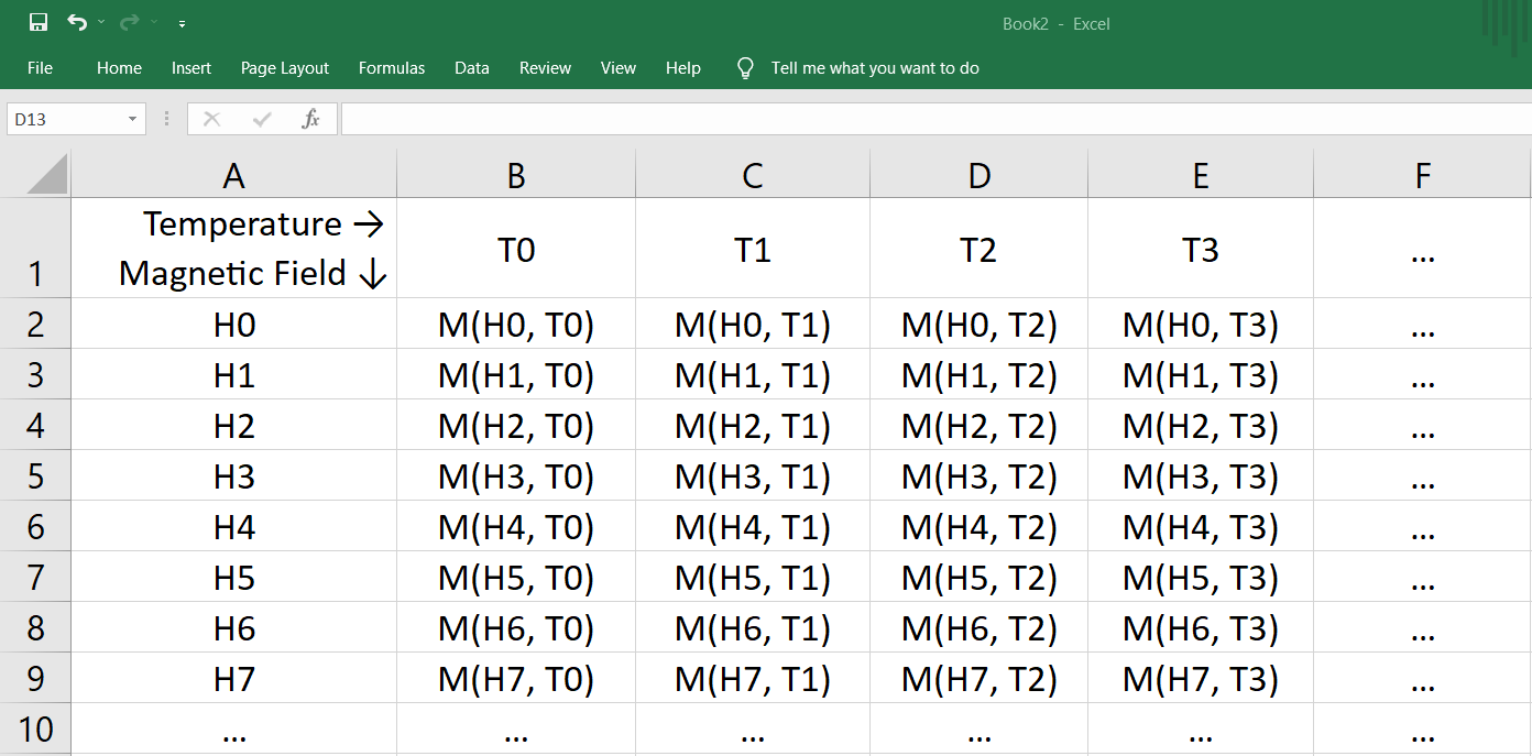
- The first row and column should contain temperature and applied magnetic field values.
- Fill the corresponding cells with numeric float values (do not use any alphabetic characters).
- Optionally, you can add an extra magnetic field value (`Hmax + del_H`) with null magnetic moment values. This helps align the magnetic moment values of the last row for calculation but is not necessary.
### 2. Execution
To utilize the functions in **magnetocaloric**, follow these steps:
one can structure the code in a class called mceanalysis to provide a unified interface for using the functions from the mcepy module :
```python
from magnetocaloric import mcepy as mp
class mceanalysis:
def __init__(self, **kwargs):
self.kwargs = kwargs
def run_interpolation(self):
mp.interpol(**self.kwargs)
def plot_mce_data(self):
mp.mce(**self.kwargs)
def plot_mce_3d_data(self):
mp.mce_3d(**self.kwargs)
```
To interpolate the Magnetic Moment data within a user-defined range of field values and a specified interval, the `interpol` function is available. This function offers flexibility by allowing users to set arguments such as `interpol_type`, `interpol_mode` and `degree` for interpolation with minimal error.
```python
interpolator = mceanalysis(
path='D:\python\interpolation\mce_example.xlsx',
sheet_index=1,
T_row=1,
H_col='A',
int_val=0,
final_val=50000,
interval=500,
interpol_type='lin',
interpol_mode='None',
deg='None'
)
interpolator.run_interpolation()
```
Explanation of the `interpol` function parameters:
- `path`: Specify the path to your Excel spreadsheet containing M-H data.
- `sheet_index`: Set the spreadsheet index within the Excel file.
- `T_row` and `H_col`: Specify the row and column for actual temperature and field values.
- `int_val`: Set the initial value of the applied magnetic field (H).
- `final_val`: Define the maximum applied field value for data interpolation.
- `interval`: Set the interval for interpolation.
- `interpol_type`: Choose the interpolation type. For linear interpolation, use `'lin'`. For polynomial interpolation, use `'poly'`.
- `interpol_mode`: For polynomial interpolation, choose between `'auto'` (automatically finds the best degree) or `'manual'` (set the degree manually using the `deg` argument).
- `deg`: If using manual polynomial interpolation, specify the degree as an integer.
> **Warning**
The interpolated data will overwrite the source file specified in the `path`. Exercise caution when using this function.
#### Example: Polynomial Interpolation with Different Degrees
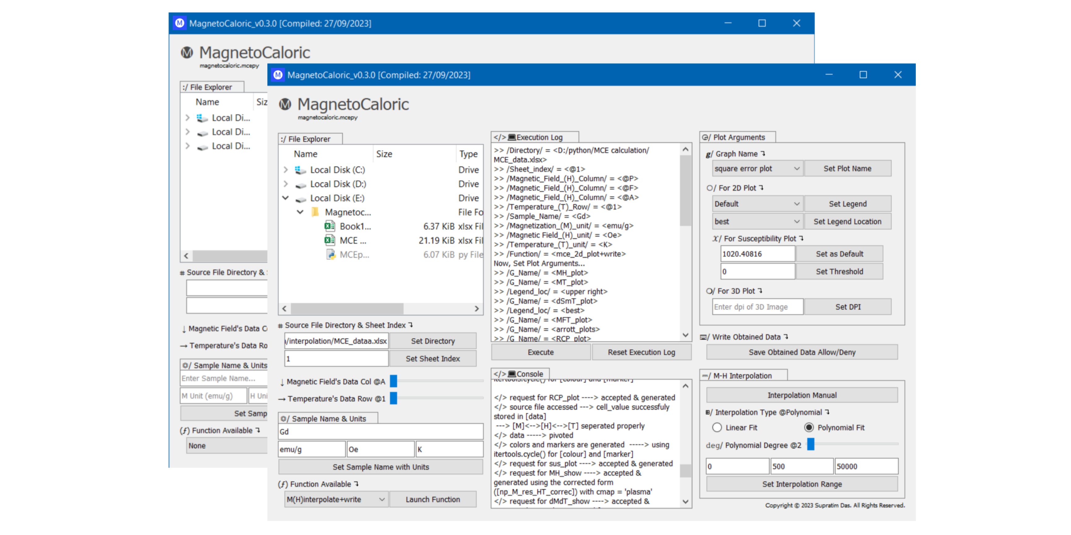
You can perform polynomial interpolation with different degrees using the **magnetocaloric** module. In this example, we'll interpolate the data with degree 3 and visualize the results. The image provided below demonstrates the square error of the interpolated data when compared to the original provided data. By visualizing this error, users can easily determine the degree at which the interpolation minimizes error while using polynomial interpolation. Lower error values signify a better fit, indicating that the chosen degree provides a closer approximation to the original data. This graphical representation helps users make informed decisions about the appropriate degree for their specific data sets, ultimately ensuring accurate and reliable results.
```python
interpolator = mceanalysis(
path='D:/python/interpolation/MCE_example.xlsx',
sheet_index=1,
T_row=1,
H_col='A',
int_val=0,
final_val=50000,
interval=500,
interpol_type='poly',
interpol_mode='manual',
deg=3 # To visualize with degree 2, change to deg=2
)
interpolator.run_interpolation()
```
Here, you can compare the interpolation results for different degrees in the following image:

### Using the `mce` Function for Customizable Graphs
The **magnetocaloric** module provides a versatile `mce` function that allows you to plot various graphs with high customization. Here's how you can use it:
```python
plotter = mceanalysis(
samp_name="unknown",
file_dir='D:\python\mce_example.xlsx',
sheet_index=1,
T_row=1,
H_col='A',
g_name='dSmT_plot',
M_unit='emu/g',
H_unit='Oe',
T_unit='K',
plot_legend='Yes',
loc='upper right',
field='None',
linear_threshold='None',
save_data='allow'
)
plotter.plot_mce_data()
```
Explanation of the function parameters:
- `samp_name`: Specify the sample name or identifier.
- `file_dir`: Provide the source data directory (Excel file path).
- `sheet_index`: Set the spreadsheet index within the Excel file.
- `T_row` and `H_col`: Specify the row and column for actual temperature and field values.
- `g_name`: Set the graph identity from the options listed above.
- `M_unit`, `H_unit`, `T_unit`: Define the units for magnetic moment, magnetic field, and temperature, respectively.
- `plot_legend` and `loc`: Decide whether to display legends on the graph and their position.
- `field` and `linear_threshold`: These are specific to susceptibility graph plotting. `field` specifies the field value for plotting susceptibility, and `linear_threshold` (range: -1 to +1) adjusts the linear regression for finding the Curie-Weiss temperature.
- `save_data`: Allow or disallow the saving of calculated data in new files.
> **Note**
The `field` and `linear_threshold` arguments are used for susceptibility graph plotting. Unless you need to plot susceptibility or all graphs together, you can leave them as 'None'.
#### Example: Susceptibility and Inverse Susceptibility Plotting
In this example, we will plot the susceptibility and inverse susceptibility by specifying the field and adjusting the linear threshold for a precise fit.
```python
plotter = mceanalysis(
samp_name="unknown",
file_dir='D:/python/MCE calculation/MCE_example.xlsx',
sheet_index=1,
T_row=1,
H_col='A',
g_name='sus_plot',
M_unit='emu/g',
H_unit='Oe',
T_unit='K',
plot_legend='Yes',
loc='upper right',
field='1020.40816',
linear_threshold=0.9995,
save_data='allow'
)
plotter.plot_mce_data()
```
In this case, we set the `linear_threshold` near unity to achieve the best linear fit in the higher temperature linear inverse susceptibility region (Curie-Weiss region).

### Using the `mce_3d` Function for 3D Data Visualization
The **magnetocaloric** module provides a powerful `mce_3d` function for visualizing data distribution in 3D. Here's how you can use it:
```python
plotter_3d = mceanalysis(
path="D:/python/MCE calculation/MCE_example.xlsx",
sheet_index=1,
T_row=1,
H_col='A',
g_name='dSm_show',
M_unit='emu/g',
H_unit='Oe',
T_unit='K',
dpi=1600,
save_data='allow'
)
plotter_3d.plot_mce_3d_data()
```
Explanation of the function parameters:
- `path`: Specify the path to the Excel file containing the data.
- `sheet_index`: Set the spreadsheet index within the Excel file.
- `T_row` and `H_col`: Specify the row and column for actual temperature and field values.
- `g_name`: Choose the type of 3D data distribution you want to visualize. Options include those provided above.
- `M_unit`, `H_unit`, `T_unit`: Define the units for magnetic moment, magnetic field, and temperature, respectively.
- `sheet_index`: Set the spreadsheet index within the Excel file.
- `T_row` and `H_col`: Specify the row and column for actual temperature and field values.
- `dpi`: Adjust the resolution of the distribution image.
- `save_data`: Allow or disallow the saving of calculated data in new files.
#### Example: Magnetic Moment (M) Distribution in 3D
In this example, we visualize the magnetic moment (M) distribution in 3D. The resulting image allows you to view the distribution from different perspectives.

## Contributing
### We Welcome Your Contributions!
If you're interested in contributing to the development of this project, your contributions are highly appreciated. Whether you find a bug, have an idea for a new feature, or want to improve the code, you can do so by raising an issue or pull request on our GitHub repository. Your input helps make this project better for everyone.
Feel free to explore the code, try out the application, and share your thoughts with us. We value the contributions of our community members and look forward to collaborating with you. Let's make this project even more amazing together!
### Contact Information:
If you have any questions or need assistance, you can reach out to me directly via email at supratim0707@gmail.com.
Raw data
{
"_id": null,
"home_page": "https://github.com/supratimdasinfo/magnetocaloric.mcepy",
"name": "magnetocaloric",
"maintainer": "",
"docs_url": null,
"requires_python": "",
"maintainer_email": "",
"keywords": "magnetocaloric,software,mcepy,magnetic,programming,code,python,supratim,das,physics",
"author": "Supratim Das",
"author_email": "supratim0707@gmail.com",
"download_url": "https://files.pythonhosted.org/packages/1e/3c/39c7605c66be639f5f3fd0dd2d64629052305091ad70258ef32e453b9c6b/magnetocaloric-1.7.1.tar.gz",
"platform": null,
"description": "# Magnetocaloric - Python Module for Magnetocaloric Performance Analysis\r\n\r\n\r\n\r\n[](https://pepy.tech/project/magnetocaloric)\r\n\r\n\r\n\r\n\r\n\r\n\r\n\r\n\r\n## Overview\r\n\r\n**magnetocaloric** is a powerful Python module designed to determine the magnetocaloric performance of magnetic materials. Developed by Supratim Das, this module provides an effective way to analyze magnetic behavior and parameters using isotherm M(H) curves and the Maxwell Relation.\r\n\r\n## Key Features\r\n\r\n- Import M-H data from XLSX files.\r\n- Interpolate magnetic moment polynomially or linearly for precise analysis and visualization.\r\n- Generate various insightful graphs, including:\r\n\r\n| Graph Description | g_name |\r\n|--------------------------------------------|-------------------|\r\n| M vs H (Magnetization vs Magnetic Field) | `MH_plot` |\r\n| M vs T (Magnetization vs Temperature) | `MT_plot` |\r\n| Entropy Change vs T | `dSmT_plot` |\r\n| Mean Field Arrott Plot | `MFT_plot` |\r\n| Temperature depedence of N exponent | `N_plot` |\r\n| Modified Arrott's Plot | `arrott_plots` |\r\n| Susceptibility and Inverse Susceptibility vs T | `sus_plot` |\r\n| Relative Cooling Power | `RCP_plot` |\r\n\r\nThis table provides a clear and concise overview of the various graphs and their corresponding `g_name` in your Python module.\r\n- Combine and visualize all graphs at once using `all_plots`.\r\n- Save calculated data for future use with the `save_data` option.\r\n- Automatically create an output folder to store results as XLSX files in the source file's directory.\r\n- Visualize 3D models of:\r\n\r\n| 3D Model Description | g_name |\r\n|------------------------------------------------------------|-----------------|\r\n| Magnetization distribution | `MH_show` |\r\n| dM/dT distribution | `dMdT_show` |\r\n| dM/dH distribution | `dMdH_show` |\r\n| Entropy change distribution for comprehensive data analysis | `dSm_show` |\r\n| d^2M/(dT.dH) distribution | `d2MdTH_show` |\r\n\r\nThis table provides a clear and concise overview of the 3D models and their corresponding `g_name`.\r\n\r\n- Intuitive Graphical User Interface: Simplifying Program Interaction. Experience seamless interaction with our PyQt5-powered UI. Standalone Python executable created using PyInstaller - no additional dependencies required.\r\n\r\n\r\n\r\nFor the Python programming approach, follow the steps in the README.\r\n\r\n## Installation\r\n\r\nYou can easily install the **magnetocaloric** package using pip. Open your command-line interface and run the following command:\r\n\r\n```shell\r\npip install magnetocaloric==1.7.1\r\n```\r\n\r\nThis will install the specified version of the **magnetocaloric** package.\r\n\r\n\r\n## Examples of How To Use\r\n\r\n### 1. Managing Excel Spreadsheet\r\n\r\nBefore using the **magnetocaloric** module, ensure that your Excel spreadsheet follows this specific format for M-H data:\r\n\r\n\r\n\r\n- The first row and column should contain temperature and applied magnetic field values.\r\n- Fill the corresponding cells with numeric float values (do not use any alphabetic characters).\r\n- Optionally, you can add an extra magnetic field value (`Hmax + del_H`) with null magnetic moment values. This helps align the magnetic moment values of the last row for calculation but is not necessary.\r\n\r\n### 2. Execution\r\n\r\nTo utilize the functions in **magnetocaloric**, follow these steps:\r\n\r\none can structure the code in a class called mceanalysis to provide a unified interface for using the functions from the mcepy module :\r\n\r\n```python\r\nfrom magnetocaloric import mcepy as mp\r\n\r\nclass mceanalysis:\r\n def __init__(self, **kwargs):\r\n self.kwargs = kwargs\r\n\r\n def run_interpolation(self):\r\n mp.interpol(**self.kwargs)\r\n \r\n def plot_mce_data(self):\r\n mp.mce(**self.kwargs)\r\n\r\n def plot_mce_3d_data(self):\r\n mp.mce_3d(**self.kwargs)\r\n \r\n```\r\nTo interpolate the Magnetic Moment data within a user-defined range of field values and a specified interval, the `interpol` function is available. This function offers flexibility by allowing users to set arguments such as `interpol_type`, `interpol_mode` and `degree` for interpolation with minimal error. \r\n\r\n```python\r\ninterpolator = mceanalysis(\r\n path='D:\\python\\interpolation\\mce_example.xlsx',\r\n sheet_index=1,\r\n T_row=1,\r\n H_col='A',\r\n int_val=0,\r\n final_val=50000,\r\n interval=500,\r\n interpol_type='lin',\r\n interpol_mode='None',\r\n deg='None'\r\n)\r\n\r\ninterpolator.run_interpolation()\r\n\r\n```\r\n\r\nExplanation of the `interpol` function parameters:\r\n\r\n- `path`: Specify the path to your Excel spreadsheet containing M-H data.\r\n- `sheet_index`: Set the spreadsheet index within the Excel file.\r\n- `T_row` and `H_col`: Specify the row and column for actual temperature and field values.\r\n- `int_val`: Set the initial value of the applied magnetic field (H).\r\n- `final_val`: Define the maximum applied field value for data interpolation.\r\n- `interval`: Set the interval for interpolation.\r\n- `interpol_type`: Choose the interpolation type. For linear interpolation, use `'lin'`. For polynomial interpolation, use `'poly'`.\r\n- `interpol_mode`: For polynomial interpolation, choose between `'auto'` (automatically finds the best degree) or `'manual'` (set the degree manually using the `deg` argument).\r\n- `deg`: If using manual polynomial interpolation, specify the degree as an integer.\r\n\r\n> **Warning**\r\nThe interpolated data will overwrite the source file specified in the `path`. Exercise caution when using this function.\r\n\r\n#### Example: Polynomial Interpolation with Different Degrees\r\n\r\nYou can perform polynomial interpolation with different degrees using the **magnetocaloric** module. In this example, we'll interpolate the data with degree 3 and visualize the results. The image provided below demonstrates the square error of the interpolated data when compared to the original provided data. By visualizing this error, users can easily determine the degree at which the interpolation minimizes error while using polynomial interpolation. Lower error values signify a better fit, indicating that the chosen degree provides a closer approximation to the original data. This graphical representation helps users make informed decisions about the appropriate degree for their specific data sets, ultimately ensuring accurate and reliable results.\r\n\r\n\r\n```python\r\ninterpolator = mceanalysis(\r\n path='D:/python/interpolation/MCE_example.xlsx',\r\n sheet_index=1,\r\n T_row=1,\r\n H_col='A',\r\n int_val=0,\r\n final_val=50000,\r\n interval=500,\r\n interpol_type='poly',\r\n interpol_mode='manual',\r\n deg=3 # To visualize with degree 2, change to deg=2\r\n)\r\n\r\ninterpolator.run_interpolation()\r\n\r\n```\r\n\r\nHere, you can compare the interpolation results for different degrees in the following image:\r\n\r\n\r\n\r\n\r\n### Using the `mce` Function for Customizable Graphs\r\n\r\nThe **magnetocaloric** module provides a versatile `mce` function that allows you to plot various graphs with high customization. Here's how you can use it:\r\n\r\n```python\r\nplotter = mceanalysis(\r\n samp_name=\"unknown\",\r\n file_dir='D:\\python\\mce_example.xlsx',\r\n sheet_index=1,\r\n T_row=1,\r\n H_col='A',\r\n g_name='dSmT_plot',\r\n M_unit='emu/g',\r\n H_unit='Oe',\r\n T_unit='K',\r\n plot_legend='Yes',\r\n loc='upper right',\r\n field='None',\r\n linear_threshold='None',\r\n save_data='allow'\r\n)\r\n\r\nplotter.plot_mce_data()\r\n\r\n```\r\n\r\nExplanation of the function parameters:\r\n\r\n- `samp_name`: Specify the sample name or identifier.\r\n- `file_dir`: Provide the source data directory (Excel file path).\r\n- `sheet_index`: Set the spreadsheet index within the Excel file.\r\n- `T_row` and `H_col`: Specify the row and column for actual temperature and field values.\r\n- `g_name`: Set the graph identity from the options listed above.\r\n- `M_unit`, `H_unit`, `T_unit`: Define the units for magnetic moment, magnetic field, and temperature, respectively.\r\n- `plot_legend` and `loc`: Decide whether to display legends on the graph and their position.\r\n- `field` and `linear_threshold`: These are specific to susceptibility graph plotting. `field` specifies the field value for plotting susceptibility, and `linear_threshold` (range: -1 to +1) adjusts the linear regression for finding the Curie-Weiss temperature.\r\n- `save_data`: Allow or disallow the saving of calculated data in new files.\r\n\r\n> **Note** \r\nThe `field` and `linear_threshold` arguments are used for susceptibility graph plotting. Unless you need to plot susceptibility or all graphs together, you can leave them as 'None'.\r\n\r\n#### Example: Susceptibility and Inverse Susceptibility Plotting\r\n\r\nIn this example, we will plot the susceptibility and inverse susceptibility by specifying the field and adjusting the linear threshold for a precise fit.\r\n\r\n```python\r\nplotter = mceanalysis(\r\n samp_name=\"unknown\",\r\n file_dir='D:/python/MCE calculation/MCE_example.xlsx',\r\n sheet_index=1,\r\n T_row=1,\r\n H_col='A',\r\n g_name='sus_plot',\r\n M_unit='emu/g',\r\n H_unit='Oe',\r\n T_unit='K',\r\n plot_legend='Yes',\r\n loc='upper right',\r\n field='1020.40816',\r\n linear_threshold=0.9995,\r\n save_data='allow'\r\n)\r\n\r\nplotter.plot_mce_data()\r\n\r\n```\r\n\r\nIn this case, we set the `linear_threshold` near unity to achieve the best linear fit in the higher temperature linear inverse susceptibility region (Curie-Weiss region).\r\n\r\n\r\n\r\n### Using the `mce_3d` Function for 3D Data Visualization\r\n\r\nThe **magnetocaloric** module provides a powerful `mce_3d` function for visualizing data distribution in 3D. Here's how you can use it:\r\n\r\n```python\r\nplotter_3d = mceanalysis(\r\n path=\"D:/python/MCE calculation/MCE_example.xlsx\",\r\n sheet_index=1,\r\n T_row=1,\r\n H_col='A',\r\n g_name='dSm_show',\r\n M_unit='emu/g',\r\n H_unit='Oe',\r\n T_unit='K',\r\n dpi=1600,\r\n save_data='allow'\r\n)\r\n\r\nplotter_3d.plot_mce_3d_data()\r\n\r\n```\r\n\r\nExplanation of the function parameters:\r\n\r\n- `path`: Specify the path to the Excel file containing the data.\r\n- `sheet_index`: Set the spreadsheet index within the Excel file.\r\n- `T_row` and `H_col`: Specify the row and column for actual temperature and field values.\r\n- `g_name`: Choose the type of 3D data distribution you want to visualize. Options include those provided above.\r\n- `M_unit`, `H_unit`, `T_unit`: Define the units for magnetic moment, magnetic field, and temperature, respectively.\r\n- `sheet_index`: Set the spreadsheet index within the Excel file.\r\n- `T_row` and `H_col`: Specify the row and column for actual temperature and field values.\r\n- `dpi`: Adjust the resolution of the distribution image.\r\n- `save_data`: Allow or disallow the saving of calculated data in new files.\r\n\r\n#### Example: Magnetic Moment (M) Distribution in 3D\r\n\r\nIn this example, we visualize the magnetic moment (M) distribution in 3D. The resulting image allows you to view the distribution from different perspectives.\r\n\r\n\r\n\r\n\r\n\r\n## Contributing\r\n### We Welcome Your Contributions!\r\n\r\nIf you're interested in contributing to the development of this project, your contributions are highly appreciated. Whether you find a bug, have an idea for a new feature, or want to improve the code, you can do so by raising an issue or pull request on our GitHub repository. Your input helps make this project better for everyone.\r\n\r\nFeel free to explore the code, try out the application, and share your thoughts with us. We value the contributions of our community members and look forward to collaborating with you. Let's make this project even more amazing together!\r\n\r\n### Contact Information: \r\n\r\nIf you have any questions or need assistance, you can reach out to me directly via email at supratim0707@gmail.com.\r\n\r\n\r\n",
"bugtrack_url": null,
"license": "MIT",
"summary": "Effective Approach To Calculate Magnetocaloric Effect Of Any Magnetic Material Using Python",
"version": "1.7.1",
"project_urls": {
"Homepage": "https://github.com/supratimdasinfo/magnetocaloric.mcepy"
},
"split_keywords": [
"magnetocaloric",
"software",
"mcepy",
"magnetic",
"programming",
"code",
"python",
"supratim",
"das",
"physics"
],
"urls": [
{
"comment_text": "",
"digests": {
"blake2b_256": "a10761835d110f55c93ecfde44c2977d053018f7ad7da291bb5cc6c201ff4ff3",
"md5": "8a3ddc0b3a29cb953e37fde636a0afe1",
"sha256": "862e1f2dd6cffd0c1b9e605298db2ab08001860801d60261ca048d0bc7a737ac"
},
"downloads": -1,
"filename": "magnetocaloric-1.7.1-py3-none-any.whl",
"has_sig": false,
"md5_digest": "8a3ddc0b3a29cb953e37fde636a0afe1",
"packagetype": "bdist_wheel",
"python_version": "py3",
"requires_python": null,
"size": 29407,
"upload_time": "2024-02-21T03:30:07",
"upload_time_iso_8601": "2024-02-21T03:30:07.983610Z",
"url": "https://files.pythonhosted.org/packages/a1/07/61835d110f55c93ecfde44c2977d053018f7ad7da291bb5cc6c201ff4ff3/magnetocaloric-1.7.1-py3-none-any.whl",
"yanked": false,
"yanked_reason": null
},
{
"comment_text": "",
"digests": {
"blake2b_256": "1e3c39c7605c66be639f5f3fd0dd2d64629052305091ad70258ef32e453b9c6b",
"md5": "d35189ed3e17ea4b76eafae49a3927a4",
"sha256": "95493f92ced05481a94feabbc9685e8255059a0d61c325e36782410ac1f342b7"
},
"downloads": -1,
"filename": "magnetocaloric-1.7.1.tar.gz",
"has_sig": false,
"md5_digest": "d35189ed3e17ea4b76eafae49a3927a4",
"packagetype": "sdist",
"python_version": "source",
"requires_python": null,
"size": 26690,
"upload_time": "2024-02-21T03:30:11",
"upload_time_iso_8601": "2024-02-21T03:30:11.424792Z",
"url": "https://files.pythonhosted.org/packages/1e/3c/39c7605c66be639f5f3fd0dd2d64629052305091ad70258ef32e453b9c6b/magnetocaloric-1.7.1.tar.gz",
"yanked": false,
"yanked_reason": null
}
],
"upload_time": "2024-02-21 03:30:11",
"github": true,
"gitlab": false,
"bitbucket": false,
"codeberg": false,
"github_user": "supratimdasinfo",
"github_project": "magnetocaloric.mcepy",
"travis_ci": false,
"coveralls": false,
"github_actions": false,
"lcname": "magnetocaloric"
}

