[ChangeLog](CHANGE_LOG.rst)
# pyg2p
pyg2p is a converter between GRIB and netCDF4/PCRaster files.
It can also manipulates GRIB messages (performing aggregation or simple unit conversion) before to apply format conversion.
## Installation
To install package, you can use a python virtual environment or directly install dependencies and
package at system level (executable script will be saved into /usr/local/bin in this case).
### Using miniconda:
* Install [miniconda](https://docs.conda.io/en/latest/miniconda.html)
* Create a conda env named "pyg2penv" and install dependencies:
```bash
conda create --name pyg2penv python=3.7 -c conda-forge
conda activate pyg2penv
```
>IMPORTANT: Before to launch setup, you need the following steps:
>Install eccodes (and GDAL): this can be done compiling from source code or using the available conda virtual environment package by running
```bash
$ conda install -c conda-forge gdal eccodes
```
>Configure geopotentials and intertables paths in
configuration/global/global_conf.json. These paths are used by pyg2p to read
geopotentials and intertables already configured. You may need to download files from FTP (launch `pyg2p -W` for this).
Users running pyg2p installed by a different user (ie. root) will configure similar paths for their own intertables
and geopotentials under his home folder. These paths will need write permissions.
Grab last archive and extract it in a folder (or clone this repository) and follow these steps:
```bash
$ cd pyg2p
$ vim configuration/global/global_conf.json # to edit shared paths !!!
$ pip install -r requirements.txt
$ pip install .
```
After installation, you will have all dependencies installed and an executable script 'pyg2p' (in a
virtual environment, script is located under <VIRTUALENV_PATH>/bin folder otherwise under
/usr/local/bin). To check correct installation of eccodes run the following command:
```bash
$ python -m eccodes selfcheck
```
Some python packages can be problematic to install at first shot. Read
following paragraph for details.
## Configuration
One of the things to configure for any user running pyg2p, is GEOPOTENTIALS and INTERTABLES
variables with paths to folders with write permissions.
>NOTE: From version 2.1, the user needs to setup these variables only if she/he
needs to write new interpolation tables (option -B [-X]) or to add new
geopotentials from grib files (option -g).
These variables contains user paths and must be configured in a .conf file (e.g. paths.conf) under
~/.pyg2p/ directory. This can look like:
```text
GEOPOTENTIALS=/dataset/pyg2p_data_user/geopotentials
INTERTABLES=/dataset/pyg2p_data_user/intertables
```
User intertables (for interpolation) are read/write from `INTERTABLES` and geopotentials (for
correction) are read from `GEOPOTENTIALS`.
Pyg2p will use its default configuration for available intertables and geopotentials. These are read
from paths configured during installation in global_conf.json.
If you need to download default files from ECMWF FTP, just launch pyg2p with -W option and the
dataset argument (argument can be *geopotentials* or *intertables*) and files are saved in user
paths configured above:
```bash
$ pyg2p -W intertables
```
You can edit FTP authentication parameters in *~/.pyg2p/ftp.json*
### Advanced configuration
User json configuration files are empty. If you need a new parameter or geopotential that is not
configured internally in pyg2p, you can setup new items (or overwrite internal configuration).
#### Adding a parameter to ~/.pyg2p/parameters.json
If you are extracting a parameter with shortName xy from a grib file that is not already globally
configured, add an element as shown below (only part in bold has been added):
```json
{
"xy": {
"@description": "Variable description",
"@shortName": "xy",
"@unit": "unitstring"
}
}
```
You can configure (more than) a conversion element with different ids and functions. You will use
shortName and conversionId in the execution JSON templates.
```json
{
"xy": { "@description": "Variable description",
"@shortName": "xy",
"@unit": "unitstring"
},
"xyz": {
"@description": "Variable description",
"@shortName": "xyz",
"@unit": "unitstring/unistring2",
"Conversion": [
{
"@cutOffNegative": true,
"@function": "x=x*(-0.13)**2",
"@id": "conv_xyz1",
"@unit": "g/d"
},
{
"@cutOffNegative": true,
"@function": "x=x/5466 - (x**2)",
"@id": "conv_xyz2",
"@unit": "g/h"
}
]
}
}
```
>Note: Aware the syntax of conversion functions. They must start with x= followed
by the actual conversion formula where x is the value to convert. Units are only
used for logging.
#### Adding a geopotential for correction
If the input grib file has a geopotential message, pyg2p will use it for correction. Otherwise, it will
read the file from user data paths or global data paths.
To add a geopotential GRIB file to pyg2p configuration, use this command:
```bash
$ pyg2p -g path_to_geopotential_grib
```
This will copy the file to folder defined in `GEOPOTENTIALS` variable and will update
geopotentials.json with the new item.
#### Interpolation tables
Interpolation tables are read from user or global data folders.
If the table is missing, it will create it into user data folder for future interpolations (you must pass
-B option to pyg2p).
Depending on source and target grids size, and on interpolation method, table creation can take
from minutes to days. To speed up interpolation table creation, use parallel option -X to have up to
x6 speed gain.
### Execution templates
Execution templates are JSON files that you will use to configure a conversion. You will pass path to
the file to pyg2p with command line option `-c`.
Most of options can be both defined in this JSON file and from command line.
**Note that command line options overwrite JSON template.**
If you have a large set of conversions for same parameters, it's more convenient to define a single
template where you define parameter, interpolation and aggregation and pass the rest of parameters from command line.
Here some examples of JSON commands files:
```json
{
"Execution": {
"@name": "Octahedral test 1",
"Aggregation": {
"@step": 24,
"@type": "average"
},
"OutMaps": {
"@cloneMap": "/dataset/maps/europe5km/dem.map",
"@ext": 1,
"@fmap": 1,
"@namePrefix": "t2",
"@unitTime": 24,
"Interpolation": {
"@latMap": "/dataset/maps/europe5km/lat.map",
"@lonMap": "/dataset/maps/europe5km/long.map",
"@mode": "grib_nearest"
}
},
"Parameter": {
"@applyConversion": "k2c",
"@correctionFormula": "p+gem-dem*0.0065",
"@demMap": "/dataset/maps/europe5km/dem.map",
"@gem": "(z/9.81)*0.0065",
"@shortName": "2t"
}
}
}
```
There are four sections of configuration.
#### Aggregation
Defines the aggregation method and step. Method can be `accumulation`, `average` or `instantaneous`.
#### OutMaps
Here you define interpolation method and paths to coordinates netCDF/PCRaster maps, output unit time, the clone map etc.
#### Interpolation
This is a subelement of OutMaps. Here you define interpolation method (see later for details), paths
to coordinates maps.
#### Parameter
In this section, you configure the parameter to select by using its shortName, as stored in GRIB file.
You also configure conversion with applyConversion property set to a conversion id. Parameter
shortName must be already configured in `~/.pyg2p/parameters.json` along with conversion ids.
If you need to apply correction based on DEM files and geopotentials, you can configure formulas
and the path to DEM map.
#### Path configuration
You can use variables in JSON files to define paths. Variables can be configured in `.conf` files under
~/.pyg2p/ folder.
`/home/domenico/.pyg2p/myconf.conf`
```console
EUROPE_MAPS=/dataset/maps/europe5km
DEM_MAP=/dataset/maps/dem05.map
EUROPE_DEM=/dataset/maps/europe/dem.map
EUROPE_LAT=/dataset/maps/europe/lat.map
EUROPE_LON=/dataset/maps/europe/long.map
```
Usage of user defined paths in JSON command file:
```json
{
"Execution": {
"@name": "eue_t24",
"Aggregation": {
"@step": 24,
"@type": "average"
},
"OutMaps": {
"@format": "netcdf",
"@cloneMap": "{EUROPE_MAPS}/lat.map",
"@ext": 1,
"@fmap": 1,
"@namePrefix": "pT24",
"@unitTime": 24,
"Interpolation": {
"@latMap": "{EUROPE_MAPS}/lat.map",
"@lonMap": "{EUROPE_MAPS}/long.map",
"@mode": "grib_nearest"
}
},
"Parameter": {
"@applyConversion": "k2c",
"@correctionFormula": "p+gem-dem*0.0065",
"@demMap": "{DEM_MAP}",
"@gem": "(z/9.81)*0.0065",
"@shortName": "2t"
}
}
}
```
### Full list of options
<table>
<thead>
<tr>
<th>Section</th>
<th>Attribute</th>
<th>Description</th>
</tr>
</thead>
<tbody>
<tr>
<td><b>Execution</b></td>
<td>name</td>
<td>Descriptive name of the execution configuration.</td>
</tr>
<tr>
<td> </td><td>intertableDir</td><td>Alternative home folder for interpolation lookup
tables, where pyg2p will load/save intertables. Folder must be existing. If not set, pyg2p will use intertables from ~/.pyg2p/intertables/</td>
</tr>
<tr>
<td> </td><td>geopotentialDir</td><td>Alternative home folder for geopotential lookup
tables. Folder must be existing. If not set, pyg2p will use geopotentials from ~/.pyg2p/geopotentials/</td>
</tr>
<tr>
<td></td><td><b>Parameter</b></td><td>See relative table</td>
</tr>
<tr>
<td></td><td><b>OutMaps</b></td><td>See relative table</td>
</tr>
<tr>
<td></td><td><b>Parameter</b></td><td>See relative table</td>
</tr>
<tr>
<td colspan="3"><hr/></td>
</tr>
<tr>
<td><b>Parameter</b></td><td><b>shortName</b></td><td>The short name of the parameter, as it is in the grib file. The application use this to select messages. Must be configured in the parameters.json file, otherwise the application exits with an error.</td>
</tr>
<tr>
<td> </td><td>tstart</td><td rowspan="6">Optional grib selectors perturbationNumber,
tstart, tend, dataDate and dataTime can also be
issued via command line arguments (-m, -s, -e,
-D, -T), which overwrite the ones in the
execution JSON file.</td>
</tr>
<tr>
<td> </td><td>tend</td>
</tr>
<tr>
<td> </td><td>perturbationNumber</td>
</tr>
<tr>
<td> </td><td>dataDate</td>
</tr>
<tr>
<td> </td><td>dataTime</td>
</tr>
<tr>
<td> </td><td>level</td>
</tr>
<tr><td> </td><td>applyConversion</td><td>The conversion id to apply, as in the
parameters.json file for the parameter to select.
The combination parameter/conversion must be
properly configured in parmaters.json file,
otherwise the application exits with an error.</td></tr>
<tr><td> </td><td>correctionFormula</td><td>Formula to use for parameter correction with p,
gem, dem variables, representing parameter
value, converted geopotential to gem, and DEM
map value. E.g.: p+gem*0.0065-dem*0.0065</td></tr>
<tr><td> </td><td>demMap</td><td>The dem map used for correction.</td></tr>
<tr><td> </td><td>gem</td><td>Formula for geopotential conversion for
correction.</td></tr>
<tr>
<td colspan="3"><hr/></td>
</tr>
<tr>
<td><b>OutMaps</b></td><td>cloneMap</td><td>The clone map with area (must have a REAL cell
type and missing values for points outside area
of interest. A dem map works fine. A typical area boolean map will not).</td>
</tr>
<tr>
<td> </td><td><b>unitTime</b></td><td>Time unit in hours of output maps. Tipical value
is 24 (daily maps). Used in "accumulation" operation</td>
</tr>
<tr>
<td> </td><td><b>format</b></td><td>Output file format. Default 'pcraster'. Available
formats are 'pcraster', 'netcdf'.</td>
</tr>
<tr>
<td> </td><td><b>namePrefix</b></td><td>Prefix for maps. Default is parameter
shortName.</td>
</tr>
<tr>
<td> </td><td><b>scaleFactor</b></td><td>Scale factor of the output netCDF map. Default 1.</td>
</tr>
<tr>
<td> </td><td><b>offset</b></td><td>Offset of the output netCDF map. Default 0.</td>
</tr>
<tr>
<td> </td><td><b>validMin</b></td><td>Minimum value of the output netCDF map. Values below will be set to nodata.</td>
</tr>
<tr>
<td> </td><td><b>validMax</b></td><td>Maximum value of the output netCDF map. Values above will be set to nodata.</td>
</tr>
<tr>
<td> </td><td><b>valueFormat</b></td><td>Variable type to use in the output netCDF map. Deafult f8. Available formats are: i1,i2,i4,i8,u1,u2,u4,u8,f4,f8 where i is integer, u is unsigned integer, f if float and the number corresponds to the number of bytes used (e.g. i4 is integer 32bits = 4 bytes)</td>
</tr>
<tr>
<td> </td><td><b>outputStepUnits</b></td><td>Step units to use in output map. If not specified, it will use the stepUnits of the source Grib file. Available values are: 's': seconds, 'm': minutes, 'h': hours, '3h': 3h steps, '6h': 6h steps, '12h': 12h steps, 'D': days</td>
</tr>
<tr>
<tr>
<td> </td><td><b>fmap</b></td><td>First PCRaster map number. Default 1.</td>
</tr>
<tr>
<td> </td><td><b>ext</b></td><td>Extension mode. It's the integer number
defining the step numbers to skip when writing PCRaster maps. Same as old grib2pcraster. Default 1.</td>
</tr>
<tr>
<td> </td><td><b>Interpolation</b></td><td>See relative table.</td>
</tr>
<tr>
<td colspan="3"><hr/></td>
</tr>
<tr>
<td><b>Aggregation</b></td><td><b>step</b></td><td>Step of aggregation in hours.</td>
</tr>
<tr>
<td> </td><td><b>type</b></td><td>Type of aggregation (it was Manipulation in
grib2pcraster). It can be average or accumulation.</td>
</tr>
<tr>
<td> </td><td><b>halfweights</b></td><td>If set to true and type is "average", it will avaluate the average by using half weights for the first and the last step</td>
</tr>
<tr>
<td> </td><td>forceZeroArray</td><td>Optional. In case of “accumulation”, and only
then, if this attribute is set to”y” (or any value different from “false”, “False”, “FALSE”, “no”,
“NO”, “No”, “0”), the program will use a zero array as message at step 0 to compute the first
map, even if the GRIB file has a step 0 message.</td>
</tr>
<tr>
<td><b>Interpolation</b></td><td><b>mode</b></td><td>Interpolation mode. Possible values are:
“nearest”, “invdist”, “grib_nearest”,
“grib_invdist”</td>
</tr>
<tr>
<td> </td><td><b>latMap</b></td><td>PCRaster map of target latitudes.</td>
</tr>
<tr>
<td> </td><td><b>lonMap</b></td><td>PCRaster map of target longitudes.</td>
</tr>
</tbody>
</table>
## Usage
To use the application, after the main configuration you need to configure a template JSON file for
each type of extraction you need to perform.
### Grabbing information from GRIB files.
To configure the application and compile your JSON templates, you might need to know the variable
shortName as stored in the input GRIB file you're using or in the geopotential GRIB. Just execute the
following GRIB tool command:
`grib_get -p shortName /path/to/grib`
Other keys you would to know for configuration or debugging purposes are:
* startStep
* endStep (for instantaneous messages, it can be the same of startStep)
* perturbationNumber (the EPS member number)
* stepType (type of field: instantaneous: 'instant', average: 'avg', cumulated: 'cumul')
* longitudeOfFirstGridPointInDegrees
* longitudeOfLastGridPointInDegrees
* latitudeOfFirstGridPointInDegrees
* latiitudeOfLastGridPointInDegrees
* Ni (it can be missing)
* Nj (it states the resolution: it's the number of points along the meridian)
* numberOfValues
* gridType (e.g.: regular_ll, reduced_gg, rotated_ll)
### Input arguments
If you run pyg2p without arguments, it shows help of all input arguments.
```console
usage: pyg2p [-h] [-c json_file] [-o out_dir] [-i input_file]
[-I input_file_2nd] [-s tstart] [-e tend] [-m eps_member]
[-T data_time] [-D data_date] [-f fmap] [-F format]
[-x extension_step] [-n outfiles_prefix] [-O offset]
[-S scale_factor] [-vM valid_max] [-vm valid_min]
[-vf value_format] [-U output_step_units] [-l log_level]
[-N intertable_dir] [-G geopotential_dir] [-B] [-X]
[-g geopotential] [-W dataset]
Pyg2p: Execute the grib to netCDF/PCRaster conversion, using parameters
from CLI/json configuration.
optional arguments:
-h, --help show this help message and exit
-c json_file, --commandsFile json_file
Path to json command file
-o out_dir, --outDir out_dir
Path where output maps will be created.
-i input_file, --inputFile input_file
Path to input grib.
-I input_file_2nd, --inputFile2 input_file_2nd
Path to 2nd resolution input grib.
-s tstart, --start tstart
Grib timestep start. It overwrites the tstart in json
execution file.
-e tend, --end tend Grib timestep end. It overwrites the tend in json
execution file.
-m eps_member, --perturbationNumber eps_member
eps member number
-T data_time, --dataTime data_time
To select messages by dataTime key value
-D data_date, --dataDate data_date
<YYYYMMDD> to select messages by dataDate key value
-f fmap, --fmap fmap First map number
-F format, --format format
Output format. Available options: netcdf, pcraster.
Default pcraster
-x extension_step, --ext extension_step
Extension number step
-n outfiles_prefix, --namePrefix outfiles_prefix
Prefix name for maps
-O offset, --offset offset
Map offset
-S scale_factor, --scaleFactor scale_factor
Map scale factor
-vM valid_max, --validMax valid_max
Max valid value
-vm valid_min, --validMin valid_min
Min valid value
-vf value_format, --valueFormat value_format
output value format (default f8)
-U output_step_units, --outputStepUnits output_step_units
output step units
-l log_level, --loggerLevel log_level
Console logging level
-N intertable_dir, --intertableDir intertable_dir
Alternate interpolation tables dir
-G geopotential_dir, --geopotentialDir geopotential_dir
Alternate geopotential dir
-B, --createIntertable
Flag to create intertable file
-X, --interpolationParallel
Use parallelization tools to make interpolation
faster.If -B option is not passed or intertable
already exists it does not have any effect.
-g geopotential, --addGeopotential geopotential
Add the file to geopotentials.json configuration file,
to use for correction. The file will be copied into
the right folder (configuration/geopotentials) Note:
shortName of geopotential must be "fis" or "z"
-W dataset, --downloadConf dataset
Download intertables and geopotentials (FTP settings
defined in ftp.json)
```
#### Usage examples:
```bash
pyg2p -c ./exec1.json -i ./input.grib -o /out/dir -s 12 -e 36 -F netcdf
pyg2p -c ./exec2.json -i ./input.grib -o /out/dir -m 10 -l INFO --format netcdf
pyg2p -c ./exec3.json -i ./input.grib -I /input2ndres.grib -o /out/dir -m 10 -l DEBUG
pyg2p -g /path/to/geopotential/grib/file # add geopotential to configuration
pyg2p -t /path/to/test/commands.txt
pyg2p -h
```
```text
Note: Even if 'netcdf' format is used for output, paths to PCRaster clone/area,
latitudes and longitudes maps have to be setup in any case.
```
### Check output maps
After the execution, you can check output maps by using the PCRaster2 Aguila viewer for PCRaster
maps or the NASA Panoply3 viewer for NetCDF files.
`aguila /dataset/testdiffmaps/eueT24/pT240000.001`
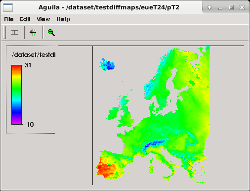
`./panoply.sh /dataset/octahedral/out/grib_vs_scipy/global/ta/p_2016-09-25_average.nc`
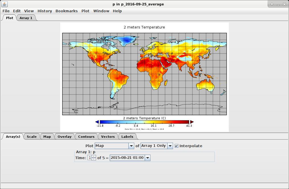
Maps will be written in the folder specified by -o input argument. If this is missing, you will find
maps in the folder where you launched the application (./).
Refer to official documentation for further information about Aguila and Panoply.
## Interpolation modes
Interpolation is configured in JSON execution templates using the *Interpolation* attribute inside
*OutMaps*.
There are four interpolation methods available. Two are using GRIB_API nearest neighbours routines
while the other two leverage on Scipy kd_tree module.
```text
Note: GRIB_API does not implement nearest neighbours routing for rotated grids.
You have to use scipy methods and regular target grids (i.e.: latitudes and
longitudes PCRaster maps).
```
### Intertable creation
Interpolation will use precompiled intertables. They will be found in the path configured in
`INTERTABLES` folder (take into account that can potentially contains gigabytes of files) or in global
data path. You can also define an alternate intertables directory with -N argument (or
*@intertableDir* attribute in JSON template).
If interlookup table doesn't exist, the application will create one into `INTERTABLES` folder and
update intertables.json configuration **only if -B option is passed**, otherwise program will exit.
Be aware that for certain combination of grid and maps, the creation of the interlookup table (which
is a numpy array saved in a binary file) could take several hours or even days for GRIB interpolation
methods.
To have better performances (up to x6 of gain) you can pass -X option to enable parallel
processing.
Performances are not comparable with scipy based interpolation (seconds or minutes) but this
option could not be viable for all GRIB inputs.
### GRIB/ecCodes API interpolation methods
To configure the interpolation method for conversion, set the @mode attribute in Execution/OutMaps/Interpolation property.
#### grib_nearest
This method uses GRIB API to perform nearest neighbour query.
To configure this method, define:
```json
{"Interpolation": {
"@latMap": "/dataset/maps/europe5km/lat.map",
"@lonMap": "/dataset/maps/europe5km/long.map",
"@mode": "grib_nearest"}
}
```
#### grib_invdist
It uses GRIB_API to query for four neighbours and relative distances. It applies inverse distance
calculation to compute the final value.
To configure this method:
```json
{
"Interpolation": {
"@latMap": "/dataset/maps/europe5km/lat.map",
"@lonMap": "/dataset/maps/europe5km/long.map",
"@mode": "grib_invdist"}
}
```
### SciPy interpolation methods
#### nearest
It's the same nearest neighbour algorithm of grib_nearest but it uses the scipy kd_tree4 module to
obtain neighbours and distances.
```json
{
"Interpolation": {
"@latMap": "/dataset/maps/europe5km/lat.map",
"@lonMap": "/dataset/maps/europe5km/long.map",
"@mode": "nearest"}
}
```
#### invdist
It's the inverse distance algorithm with scipy.kd_tree, using 4 neighbours.
```json
{
"Interpolation": {
"@latMap": "/dataset/maps/europe5km/lat.map",
"@lonMap": "/dataset/maps/europe5km/long.map",
"@mode": "invdist"}
}
```
Attributes p, leafsize and eps for the kd tree algorithm are default in scipy library:
| Attribute | Details |
|-----------|----------------------|
| p | 2 (Euclidean metric) |
| eps | 0 |
| leafsize | 10 |
#### ADW
It's the Angular Distance Weighted (ADW) algorithm by Shepard et al. 1968, with scipy.kd_tree using 11 neighbours.
If @use_broadcasting is set to true, computations will run in full broadcasting mode but requires more memory
If @num_of_splits is set to any number, computations will be split on subset and then recollected into the final map, to save mamory (do not set it if you have enought memory to run interpolation)
```json
{
"Interpolation": {
"@latMap": "/dataset/maps/europe5km/lat.map",
"@lonMap": "/dataset/maps/europe5km/long.map",
"@mode": "adw",
"@use_broadcasting": false,
"@num_of_splits": 10}
}
```
#### CDD
It's the Correlation Distance Decay (CDD) modified implementation of the Angular Distance Weighted algorithm, with scipy.kd_tree using 11 neighbours. It needs a map of CDD values for each point, to be specified in the field @cdd_map
@cdd_mode can be one of the following values: "Hofstra", "NewEtAl" or "MixHofstraShepard"
In case of mode "MixHofstraShepard", @cdd_options allows to customize the parameters of Hofstra and Shepard algorithm ("weights_mode": can be "All" or "OnlyTOP10" to take 10 higher values only in the interpolation of each point).
If @use_broadcasting is set to true, computations will run in full broadcasting mode but requires more memory
If @num_of_splits is set to any number, computations will be split on subset and then recollected into the final map, to save mamory (do not set it if you have enought memory to run interpolation)
```json
{
"Interpolation": {
"@latMap": "/dataset/maps/europe5km/lat.map",
"@lonMap": "/dataset/maps/europe5km/long.map",
"@mode": "cdd",
"@cdd_map": "/dataset/maps/europe5km/cdd_map.nc",
"@cdd_mode": "MixHofstraShepard",
"@cdd_options": {
"m_const": 4,
"min_num_of_station": 4,
"radius_ratio": 0.3333333333333333,
"weights_mode": "All"
},
"@use_broadcasting": false,
"@num_of_splits": 10}
}
```
#### bilinear
It's the bilinear interpolation algorithm applyied on regular and irregular grids. On irregular grids, it tries to get the best quatrilateral around each target point, but at the same time tries to use the best stable and grid-like shape from starting points. To do so, evaluates interpolation looking at point on similar latitude, thus on projected grib files may show some irregular results.
```json
{
"Interpolation": {
"@latMap": "/dataset/maps/europe5km/lat.map",
"@lonMap": "/dataset/maps/europe5km/long.map",
"@mode": "bilinear"}
}
```
#### triangulation
This interpolation works on a triangular tessellation of the starting grid applying the Delaunay criteria, and the uses the linear barycentric interpolation to get the target intrpolated values. It works on all type of grib files, but for some resolutions may show some edgy shapes.
```json
{
"Interpolation": {
"@latMap": "/dataset/maps/europe5km/lat.map",
"@lonMap": "/dataset/maps/europe5km/long.map",
"@mode": "triangulation"}
}
```
#### bilinear_delaunay
This algorithm merges bilinear interpolation and triangular tessellation. Quadrilaters used for the bilinear interpolation are obtained joining two adjacent triangles detected from the Delaunay triangulation of the source points. The merge is done giving priority to the ones distributed on a grid-like shape. When a quadrilateral is not available (there are no more adjacent triangles left on the grid able to merge), the linear barycentric interpolation is applyied. The result of this interpolation works smoothly and adapts automatically on all kind of source grib file.
```json
{
"Interpolation": {
"@latMap": "/dataset/maps/europe5km/lat.map",
"@lonMap": "/dataset/maps/europe5km/long.map",
"@mode": "bilinear_delaunay"}
}
```
## OutMaps configuration
Interpolation is configured under the OutMaps tag. With additional attributes, you also configure
resulting PCRaster or netCDF maps. Output dir is ./ by default or you can set it via command line using the
option -o (--outDir).
| Attribute | Details |
|----------------|-----------------------------------------------------------------------------------------------------------------------------------|
| namePrefix | Prefix name for output map files. Default is the value of shortName key. |
| unitTime | Unit time in hours for results. This is used during aggregation operations. |
| fmap | Extension number for the first map. Default 1. |
| ext | Extension mode. It's the integer number defining the step numbers to skip when writing maps. Same as old grib2pcraster. Default 1.|
| cloneMap | Path to a PCRaster clone map, needed by PCRaster libraries to write a new map on disk. |
| scaleFactor | Scale factor of the output netCDF map. Default 1. |
| offset | Offset of the output netCDF map. Default 0. |
| validMin | Minimum value of the output netCDF map. Values below will be set to nodata. |
| validMax | Maximum value of the output netCDF map. Values above will be set to nodata. |
| valueFormat | Variable type to use in the output netCDF map. Deafult f8. Available formats are: i1,i2,i4,i8,u1,u2,u4,u8,f4,f8 where i is integer, u is unsigned integer, f if float and the number corresponds to the number of bytes used (e.g. i4 is integer 32bits = 4 bytes) |
| outputStepUnits | Step units to use in output map. If not specified, it will use the stepUnits of the source Grib file. Available values are: 's': seconds, 'm': minutes, 'h': hours, '3h': 3h steps, '6h': 6h steps, '12h': 12h steps, 'D': days |
## Aggregation
Values from grib files can be aggregated before to write the final PCRaster maps. There are two kinds of aggregation available: average and accumulation.
The JSON configuration in the execution file will look like:
```json
{
"Aggregation": {
"@type": "average",
"@halfweights": false}
}
```
To better understand what these two types of aggregations do, the DEBUG output of execution is presented later in same paragraph.
### Average
Temperatures are often extracted as averages on 24 hours or 6 hours. Here's a typical execution configuration and the output of interest:
**cosmo_t24.json**
```json
{
"Execution": {
"@name": "cosmo_T24",
"Aggregation": {
"@step": 24,
"@type": "average",
"@halfweights": false
},
"OutMaps": {
"@cloneMap": "/dataset/maps/europe/dem.map",
"@ext": 4,
"@fmap": 1,
"@namePrefix": "T24",
"@unitTime": 24,
"Interpolation": {
"@latMap": "/dataset/maps/europe/lat.map",
"@lonMap": "/dataset/maps/europe/lon.map",
"@mode": "nearest"
}
},
"Parameter": {
"@applyConversion": "k2c",
"@correctionFormula": "p+gem-dem*0.0065",
"@demMap": "/dataset/maps/europe/dem.map",
"@gem": "(z/9.81)*0.0065",
"@shortName": "2t"
}
}
}
```
**Command**
`pyg2p -l DEBUG -c /execution_templates/cosmo_t24.json -i /dataset/cosmo/2012111912_pf10_t2.grb -o ./cosmo -m 10`
**ext parameter**
ext value will affect numbering of output maps:
```console
[2013-07-12 00:06:18,545] :./cosmo/T24a0000.001 written!
[2013-07-12 00:06:18,811] :./cosmo/T24a0000.005 written!
[2013-07-12 00:06:19,079] :./cosmo/T24a0000.009 written!
[2013-07-12 00:06:19,349] :./cosmo/T24a0000.013 written!
[2013-07-12 00:06:19,620] :./cosmo/T24a0000.017 written!
```
This is needed because we performed 24 hours average over 6 hourly steps.
**Details about average parameters:**
The to evaluate the average, the following steps are executed:
- when "halfweights" is false, the results of the function is the sum of all the values from "start_step-aggregation_step+1" to end_step, taking for each step the value corresponding to the next available value in the grib file. E.g:
INPUT: start_step=24, end_step=<not specified, will take the end of file>, aggregation_step=24
GRIB File: contains data starting from step 0 to 48 every 6 hours: 0,6,12,18,24,30,....
Day 1: Aggregation starts from 24-24+1=1, so it will sum up the step 6 six times, then the step 12 six times, step 18 six times, and finally the step 24 six times. The sum will be divided by the aggretation_step (24) to get the average.
Day 2: same as Day 1 starting from (24+24)-24+1=25...
- when "halfweights" is true, the results of the function is the sum of all the values from "start_step-aggregation_step" to end_step, taking for each step the value corresponding to the next available value in the grib file but using half of the weights for the first and the last step in each aggregation_step cicle. E.g:
INPUT: start_step=24, end_step=<not specified, will take the end of file>, aggregation_step=24
GRIB File: contains data starting from step 0 to 72 every 6 hours: 0,6,12,18,24,30,36,....
Day 1: Aggregation starts from 24-24=0, and will consider the step 0 value multiplied but 3, that is half of the number of steps between two step keys in the grib file. Then it will sum up the step 6 six times, then the step 12 six times, step 18 six times, and finally the step 24 again multiplied by 3. The sum will be divided by the aggretation_step (24) to get the average.
Day 2: same as Day 1 starting from (24+24)-24=24: the step 24 will have a weight of 3, while steps 30,36 and 42 will be counted 6 times, and finally the step 48 will have a weight of 3.
- if start_step is zero or is not specified, the aggregation will start from 0
### Accumulation
For precipitation values, accumulation over 6 or 24 hours is often performed. Here's an example of configuration and execution output in DEBUG mode.
**dwd_r06.json**
```json
{"Execution": {
"@name": "dwd_rain_gsp",
"Aggregation": {
"@step": 6,
"@type": "accumulation"
},
"OutMaps": {
"@cloneMap": "/dataset/maps/europe/dem.map",
"@fmap": 1,
"@namePrefix": "pR06",
"@unitTime": 24,
"Interpolation": {
"@latMap": "/dataset/maps/europe/lat.map",
"@lonMap": "/dataset/maps/europe/lon.map",
"@mode": "nearest"
}
},
"Parameter": {
"@shortName": "RAIN_GSP",
"@tend": 18,
"@tstart": 12
}
}
}
```
**Command**
`pyg2p -l DEBUG -c /execution_templates/dwd_r06.json -i /dataset/dwd/2012111912_pf10_tp.grb -o ./cosmo -m 10`
**Output**
```console
[2013-07-11 23:33:19,646] : Opening the GRIBReader for
/dataset/dwd/grib/dwd_grib1_ispra_LME_2012111900
[2013-07-11 23:33:19,859] : Grib input step 1 [type of step: accum]
[2013-07-11 23:33:19,859] : Gribs from 0 to 78
...
...
[2013-07-11 23:33:20,299] : ******** **** MANIPULATION **** *************
[2013-07-11 23:33:20,299] : Accumulation at resolution: 657
[2013-07-11 23:33:20,300] : out[s:6 e:12 res:657 step-lenght:6] = grib:12 - grib:6 *
(24/6))
[2013-07-11 23:33:20,316] : out[s:12 e:18 res:657 step-lenght:6] = grib:18 - grib:12 *
(24/6))
```
```text
Note: If you want to perform accumulation from Ts to Te with an aggregation step
Ta, and Ts-Ta=0 (e.g. Ts=6h, Te=48h, Ta=6h), the program will select the first
message at step 0 if present in the GRIB file, while you would use a zero values
message instead.
To use a zero values array, set the attribute forceZeroArray to ”true” in the
Aggregation configuration element.
For some DWD5 and COSMO6 accumulated precipitation files, the first zero message is
an instant precipitation and the decision at EFAS was to use a zero message, as it
happens for UKMO extractions, where input GRIB files don't have a first zero step
message.
```
```bash
grib_get -p units,name,stepRange,shortName,stepType 2012111912_pf10_tp.grb
kg m**-2 Total Precipitation 0 tp instant
kg m**-2 Total Precipitation 0-6 tp accum
kg m**-2 Total Precipitation 0-12 tp accum
kg m**-2 Total Precipitation 0-18 tp accum
...
...
kg m**-2 Total Precipitation 0-48 tp accum
```
## Correction
Values from grib files can be corrected with respect to their altitude coordinate (Lapse rate
formulas). Formulas will use also a geopotential value (to read from a GRIB file, see later in this
chapter for configuration).
Correction has to be configured in the Parameter element, with three mandatory attributes.
* correctionFormula (the formula used for correction, with input variables parameter value (p), gem, and dem value.
* gem (the formula to obtain gem value from geopotential z value)
* demMap (path to the DEM PCRaster map)
`Note: formulas must be written in python notation.`
Tested configurations are only for temperature and are specified as follows:
**Temperature correction**
```json
{
"Parameter": {
"@applyConversion": "k2c",
"@correctionFormula": "p+gem-dem*0.0065",
"@demMap": "/dataset/maps/europe/dem.map",
"@gem": "(z/9.81)*0.0065",
"@shortName": "2t"}
}
```
**A more complicated correction formula:**
```json
{
"Parameter": {
"@applyConversion": "k2c",
"@correctionFormula": "p/gem*(10**((-0.159)*dem/1000))",
"@demMap": "/dataset/maps/europe/dem.map",
"@gem": "(10**((-0.159)*(z/9.81)/1000))",
"@shortName": "2t"}
}
```
### How to write formulas
**z** is the geopotential value as read from the grib file
**gem** is the value resulting from the formula specified in gem attribute I.e.: (gem="(10**((-0.159)*(z/9.81)/1000)))"
**dem** is the dem value as read from the PCRaster map
Be aware that if your dem map has directions values, those will be replicated in the final map.
### Which geopotential file is used?
The application will try to find a geopotential message in input GRIB file. If a geopotential message
is not found, pyg2p will select a geopotential file from user or global data paths, by selecting
filename from configuration according the geodetic attributes of GRIB message. If it doesn't find
any suitable grib file, application will exit with an error message.
Geodetic attributes compose the key id in the JSON configuration (note the $ delimiter):
`longitudeOfFirstGridPointInDegrees$longitudeOfLastGridPointInDegrees$Ni$Nj$numberOfValues$gridType`
If you want to add another geopotential file to the configuration, just execute the command:
`pyg2p -g /path/to/geopotential/grib/file`
The application will copy the geopotential GRIB file into `GEOPOTENTIALS` folder (under user home directory)
and will also add the proper JSON configuration to geopotentials.json file.
## Conversion
Values from GRIB files can be converted before to write final output maps. Conversions are
configured in the parameters.json file for each parameter (ie. shortName).
The right conversion formula will be selected using the id specified in the *applyConversion* attribute, and the shortName
attribute of the parameter that is going to be extracted and converted.
Refer to Parameter configuration paragraph for details.
## Logging
Console logger level is INFO by default and can be optionally set by using **-l** (or **–loggerLevel**)
input argument.
Possible logger level values are ERROR, WARN, INFO, DEBUG, in increasing order of verbosity .
## pyg2p API
From version 1.3, pyg2p comes with a simple API to import and use from other python programs
(e.g. pyEfas).
The pyg2p API is intended to mimic the pyg2p.py script execution from command line so it provides
a Command class with methods to set input parameters and a *run_command(cmd)* module level function to execute pyg2p.
### Setting execution parameters
1. Create a pyg2p command:
```python
from pyg2p.main import api
command = api.command()
```
2. Setup execution parameters using a chain of methods (or single calls):
```python
command.with_cmdpath('a.json')
command.with_inputfile('0.grb')
command.with_log_level('ERROR').with_out_format('netcdf')
command.with_outdir('/dataout/').with_tstart('6').with_tend('24').with_eps('10').with_fmap('1')
command.with_ext('4')
print(str(command))
'pyg2p.py -c a.json -e 240 -f 1 -i 0.grb -l ERROR -m 10 -o /dataout/test -s 6 -x 4 -F netcdf'
```
You can also create a command object using the input arguments as you would do when execute pyg2p from command line:
```python
args_string = '-l ERROR -c /pyg2p_git/execution_templates_devel/eue_t24.json -i /dataset/test_2013330702/EpsN320-2013063000.grb -o /dataset/testdiffmaps/eueT24 -m 10'
command2 = api.command(args_string)
```
### Execute
Use the run_command function from pyg2p module. This will delegate the main method, without
shell execution.
```python
ret = api.run_command(command)
```
The function returns the same value pyg2p returns if executed from shell (0 for correct executions,
included those for which messages are not found).
### Adding geopotential file to configuration
You can add a geopotential file to configuration from pyg2p API as well, using Configuration classes:
```python
from pyg2p.main.config import UserConfiguration, GeopotentialsConfiguration
user=UserConfiguration()
geopotentials=GeopotentialsConfiguration(user)
geopotentials.add('path/to/geopotential.grib')
```
The result will be the same as executing `pyg2p -g path/to/geopotential.grib`.
### Using API to bypass I/O
Since version 3.1, pyg2p has a more usable api, useful for programmatically convert values
Here an example of usage:
```python
from pyg2p.main.api import Pyg2pApi, ApiContext
config = {
'loggerLevel': 'ERROR',
'inputFile': '/data/gribs/cosmo.grib',
'fmap': 1,
'start': 6,
'end': 132,
'perturbationNumber': 2,
'intertableDir': '/data/myintertables/',
'geopotentialDir': '/data/mygeopotentials',
'OutMaps': {
'unitTime': 24,
'cloneMap': '/data/mymaps/dem.map',
'Interpolation': {
"latMap": '/data/mymaps/lat.map',
"lonMap": '/data/mymaps/lon.map',
"mode": "nearest"
}
},
'Aggregation': {
'step': 6,
'type': 'average'
},
'Parameter': {
'shortName': 'alhfl_s',
'applyConversion': 'tommd',
},
}
ctx = ApiContext(config)
api = Pyg2pApi(ctx)
values = api.execute()
```
The `values` variable is an ordered dictionary with keys of class `pyg2p.Step`, which is simply a tuple of (start, end, resolution_along_meridian, step, level))
Each value of the dictionary is a numpy array representing a map of the converted variable for that step.
For example, the first value would correspond to a PCRaster map file <var>0000.001 generated and written by pyg2p when executed normally via CLI.
Check also this code we used in tests to validate API execution against CLI execution with same parameters:
```python
import numpy as np
from pyg2p.main.readers import PCRasterReader
for i, (step, val) in enumerate(values.items(), start=1):
i = str(i).zfill(3)
reference = PCRasterReader(f'/data/reference/cosmo/E06a0000.{i}')).values
diff = np.abs(reference - val)
assert np.allclose(diff, np.zeros(diff.shape), rtol=1.e-2, atol=1.e-3, equal_nan=True)
```
## Appendix A - Execution JSON files examples
This paragraph will explain typical execution json configurations.
### Example 1: Correction with dem and geopotentials
```shell script
pyg2p -c example1.json -i /dataset/cosmo/2012111912_pf2_t2.grb -o ./out_1
```
**example1.json**
```json
{
"Execution": {
"@name": "eue_t24",
"Aggregation": {
"@step": 24,
"@type": "average"
},
"OutMaps": {
"@cloneMap": "{EUROPE_MAPS}/lat.map",
"@ext": 1,
"@fmap": 1,
"@namePrefix": "pT24",
"@unitTime": 24,
"Interpolation": {
"@latMap": "{EUROPE_MAPS}/lat.map",
"@lonMap": "{EUROPE_MAPS}/long.map",
"@mode": "grib_nearest"
}
},
"Parameter": {
"@applyConversion": "k2c",
"@correctionFormula": "p+gem-dem*0.0065",
"@demMap": "{DEM_MAP}",
"@gem": "(z/9.81)*0.0065",
"@shortName": "2t"
}
}
}
```
This configuration, will select the 2t parameter from time step 0 to 12, out of a cosmo t2 file.
Values will be corrected using the dem map and a geopotential file as in geopotentials.json configuration.
Maps will be written under ./out_1 folder (the folder will be created if not existing yet). The clone map is set as same as dem.map.
>Note that paths to maps uses variables `EUROPE_MAPS` and `DEM_MAP`.
>You will set these variables in myconf.conf file under ~/.pyg2p/ folder.
The original values will be converted using the conversion “k2c”. This conversion must be
configured in the parameters.json file for the variable which is being extracted (2t). See Parameter
property configuration at Parameter.
The interpolation method is grib_nearest. Latitudes and longitudes values will be used only if the
interpolation lookup table (intertable) hasn't be created yet but it's mandatory to set latMap and
lonMap because the application uses their metadata raster attributes to select the right intertable.
The table filename to be read and used for interpolation is automatically found by the application,
so there is no need to specify it in configuration. However, lat and lon maps are mandatory
configuration attributes.
### Example 2: Dealing with multiresolution files
```shell script
pyg2p -c example1.json -i 20130325_en0to10.grib -I 20130325_en11to15.grib -o ./out_2
```
Performs accumulation 24 hours out of sro values of two input grib files having different vertical
resolutions. You can also feed pyg2p with a single multiresolution file.
```shell script
pyg2p -c example1.json -i 20130325_sro_0to15.grib o ./out_2 -m 0
```
```json
{
"Execution": {
"@name": "multi_sro",
"Aggregation": {
"@step": 24,
"@type": "accumulation"
},
"OutMaps": {
"@cloneMap": "/dataset/maps/global/dem.map",
"@fmap": 1,
"@namePrefix": "psro",
"@unitTime": 24,
"Interpolation": {
"@latMap": "/dataset/maps/global/lat.map",
"@lonMap": "/dataset/maps/global/lon.map",
"@mode": "grib_nearest"
}
},
"Parameter": {
"@applyConversion": "m2mm",
"@shortName": "sro",
"@tend": 360,
"@tstart": 0
}
}
}
```
This execution configuration will extract global overlapping messages sro (perturbation number 0)
from two files at different resolution.
Values will be converted using “tomm” conversion and maps (interpolation used here is
grib_nearest) will be written under ./out_6 folder.
### Example 3: Accumulation 24 hours
```shell script
./pyg2p.py -i /dataset/eue/EpsN320-2012112000.grb -o ./out_eue -c execution_file_examples/execution_9.json
```
```json
{
"Execution": {
"@name": "eue_tp",
"Aggregation": {
"@step": 24,
"@type": "accumulation"
},
"OutMaps": {
"@cloneMap": "/dataset/maps/europe5km/lat.map",
"@fmap": 1,
"@namePrefix": "pR24",
"@unitTime": 24,
"Interpolation": {
"@latMap": "/dataset/maps/europe5km/lat.map",
"@lonMap": "/dataset/maps/europe5km/long.map",
"@mode": "grib_nearest"
}
},
"Parameter": {
"@applyConversion": "tomm",
"@shortName": "tp"
}
}
}
```
## Appendix B – Netcdf format output
```prettier
Format: NETCDF4_CLASSIC.
Convention: CF-1.6
Dimensions:
xc: Number of rows of area/clone map
yc: Number of cols of area/clone map
time: Unlimited dimension for time steps
Variables:
lon: 2D array with shape (yc, xc)
lat: 2D array with shape (yc, xc)
time_nc: 1D array of values representing hours/days since dataDate of first grib message (endStep)
values_nc: a 3D array of dimensions (time, yc, xc), with coordinates set to 'lon, lat'.
```
Raw data
{
"_id": null,
"home_page": null,
"name": "pyg2p",
"maintainer": null,
"docs_url": null,
"requires_python": null,
"maintainer_email": null,
"keywords": "NetCDF GRIB PCRaster Lisflood EFAS GLOFAS",
"author": "Domenico Nappo",
"author_email": "domenico.nappo@gmail.com",
"download_url": "https://files.pythonhosted.org/packages/cc/32/35ecfd62533bb7b945f0a6a38ea831d65f1914094cd37c1012aff8d122b7/pyg2p-3.2.7.tar.gz",
"platform": null,
"description": "[ChangeLog](CHANGE_LOG.rst)\n\n\n# pyg2p\npyg2p is a converter between GRIB and netCDF4/PCRaster files. \nIt can also manipulates GRIB messages (performing aggregation or simple unit conversion) before to apply format conversion.\n\n## Installation\n\nTo install package, you can use a python virtual environment or directly install dependencies and\npackage at system level (executable script will be saved into /usr/local/bin in this case).\n\n### Using miniconda:\n\n\n* Install [miniconda](https://docs.conda.io/en/latest/miniconda.html)\n\n* Create a conda env named \"pyg2penv\" and install dependencies:\n\n ```bash\n conda create --name pyg2penv python=3.7 -c conda-forge\n conda activate pyg2penv\n ```\n\n>IMPORTANT: Before to launch setup, you need the following steps:\n\n>Install eccodes (and GDAL): this can be done compiling from source code or using the available conda virtual environment package by running \n\n```bash\n$ conda install -c conda-forge gdal eccodes\n```\n\n>Configure geopotentials and intertables paths in\nconfiguration/global/global_conf.json. These paths are used by pyg2p to read\ngeopotentials and intertables already configured. You may need to download files from FTP (launch `pyg2p -W` for this). \nUsers running pyg2p installed by a different user (ie. root) will configure similar paths for their own intertables \nand geopotentials under his home folder. These paths will need write permissions.\n\n\n\nGrab last archive and extract it in a folder (or clone this repository) and follow these steps:\n\n```bash\n$ cd pyg2p\n$ vim configuration/global/global_conf.json # to edit shared paths !!!\n$ pip install -r requirements.txt\n$ pip install .\n```\n\nAfter installation, you will have all dependencies installed and an executable script 'pyg2p' (in a\nvirtual environment, script is located under <VIRTUALENV_PATH>/bin folder otherwise under\n/usr/local/bin). To check correct installation of eccodes run the following command: \n\n```bash\n$ python -m eccodes selfcheck\n```\n\nSome python packages can be problematic to install at first shot. Read\nfollowing paragraph for details.\n\n## Configuration\n\nOne of the things to configure for any user running pyg2p, is GEOPOTENTIALS and INTERTABLES\nvariables with paths to folders with write permissions.\n\n>NOTE: From version 2.1, the user needs to setup these variables only if she/he\nneeds to write new interpolation tables (option -B [-X]) or to add new\ngeopotentials from grib files (option -g).\n\nThese variables contains user paths and must be configured in a .conf file (e.g. paths.conf) under\n~/.pyg2p/ directory. This can look like:\n\n```text\nGEOPOTENTIALS=/dataset/pyg2p_data_user/geopotentials\nINTERTABLES=/dataset/pyg2p_data_user/intertables\n```\n\nUser intertables (for interpolation) are read/write from `INTERTABLES` and geopotentials (for\ncorrection) are read from `GEOPOTENTIALS`.\nPyg2p will use its default configuration for available intertables and geopotentials. These are read\nfrom paths configured during installation in global_conf.json.\nIf you need to download default files from ECMWF FTP, just launch pyg2p with -W option and the\ndataset argument (argument can be *geopotentials* or *intertables*) and files are saved in user\npaths configured above:\n\n```bash\n$ pyg2p -W intertables\n```\n\nYou can edit FTP authentication parameters in *~/.pyg2p/ftp.json*\n\n### Advanced configuration\n\nUser json configuration files are empty. If you need a new parameter or geopotential that is not\nconfigured internally in pyg2p, you can setup new items (or overwrite internal configuration).\n\n#### Adding a parameter to ~/.pyg2p/parameters.json\n\nIf you are extracting a parameter with shortName xy from a grib file that is not already globally\nconfigured, add an element as shown below (only part in bold has been added):\n\n\n```json\n{\n \"xy\": {\n \"@description\": \"Variable description\",\n \"@shortName\": \"xy\",\n \"@unit\": \"unitstring\"\n }\n}\n```\n\nYou can configure (more than) a conversion element with different ids and functions. You will use\nshortName and conversionId in the execution JSON templates.\n\n\n```json\n{\n \"xy\": { \"@description\": \"Variable description\",\n \"@shortName\": \"xy\",\n \"@unit\": \"unitstring\"\n },\n \"xyz\": {\n \"@description\": \"Variable description\",\n \"@shortName\": \"xyz\",\n \"@unit\": \"unitstring/unistring2\",\n \"Conversion\": [\n {\n \"@cutOffNegative\": true,\n \"@function\": \"x=x*(-0.13)**2\",\n \"@id\": \"conv_xyz1\",\n \"@unit\": \"g/d\"\n },\n {\n \"@cutOffNegative\": true,\n \"@function\": \"x=x/5466 - (x**2)\",\n \"@id\": \"conv_xyz2\",\n \"@unit\": \"g/h\"\n }\n ]\n }\n}\n```\n\n>Note: Aware the syntax of conversion functions. They must start with x= followed\nby the actual conversion formula where x is the value to convert. Units are only\nused for logging.\n\n#### Adding a geopotential for correction\n\nIf the input grib file has a geopotential message, pyg2p will use it for correction. Otherwise, it will\nread the file from user data paths or global data paths.\nTo add a geopotential GRIB file to pyg2p configuration, use this command:\n\n```bash\n$ pyg2p -g path_to_geopotential_grib\n```\n\nThis will copy the file to folder defined in `GEOPOTENTIALS` variable and will update\ngeopotentials.json with the new item.\n\n#### Interpolation tables\n\nInterpolation tables are read from user or global data folders.\nIf the table is missing, it will create it into user data folder for future interpolations (you must pass\n-B option to pyg2p).\nDepending on source and target grids size, and on interpolation method, table creation can take\nfrom minutes to days. To speed up interpolation table creation, use parallel option -X to have up to\nx6 speed gain.\n\n### Execution templates\n\nExecution templates are JSON files that you will use to configure a conversion. You will pass path to\nthe file to pyg2p with command line option `-c`.\nMost of options can be both defined in this JSON file and from command line. \n**Note that command line options overwrite JSON template.**\n\nIf you have a large set of conversions for same parameters, it's more convenient to define a single\ntemplate where you define parameter, interpolation and aggregation and pass the rest of parameters from command line.\nHere some examples of JSON commands files:\n\n```json\n{\n \"Execution\": {\n \"@name\": \"Octahedral test 1\",\n \"Aggregation\": {\n \"@step\": 24,\n \"@type\": \"average\"\n },\n \"OutMaps\": {\n \"@cloneMap\": \"/dataset/maps/europe5km/dem.map\",\n \"@ext\": 1,\n \"@fmap\": 1,\n \"@namePrefix\": \"t2\",\n \"@unitTime\": 24,\n \"Interpolation\": {\n \"@latMap\": \"/dataset/maps/europe5km/lat.map\",\n \"@lonMap\": \"/dataset/maps/europe5km/long.map\",\n \"@mode\": \"grib_nearest\"\n }\n },\n \"Parameter\": {\n \"@applyConversion\": \"k2c\",\n \"@correctionFormula\": \"p+gem-dem*0.0065\",\n \"@demMap\": \"/dataset/maps/europe5km/dem.map\",\n \"@gem\": \"(z/9.81)*0.0065\",\n \"@shortName\": \"2t\"\n }\n }\n}\n```\n\nThere are four sections of configuration.\n\n#### Aggregation\nDefines the aggregation method and step. Method can be `accumulation`, `average` or `instantaneous`.\n\n#### OutMaps\nHere you define interpolation method and paths to coordinates netCDF/PCRaster maps, output unit time, the clone map etc.\n\n#### Interpolation\nThis is a subelement of OutMaps. Here you define interpolation method (see later for details), paths\nto coordinates maps.\n\n#### Parameter\nIn this section, you configure the parameter to select by using its shortName, as stored in GRIB file.\nYou also configure conversion with applyConversion property set to a conversion id. Parameter\nshortName must be already configured in `~/.pyg2p/parameters.json` along with conversion ids.\nIf you need to apply correction based on DEM files and geopotentials, you can configure formulas\nand the path to DEM map.\n\n#### Path configuration\n\nYou can use variables in JSON files to define paths. Variables can be configured in `.conf` files under\n~/.pyg2p/ folder.\n`/home/domenico/.pyg2p/myconf.conf`\n\n```console\nEUROPE_MAPS=/dataset/maps/europe5km\nDEM_MAP=/dataset/maps/dem05.map\nEUROPE_DEM=/dataset/maps/europe/dem.map\nEUROPE_LAT=/dataset/maps/europe/lat.map\nEUROPE_LON=/dataset/maps/europe/long.map\n```\n\nUsage of user defined paths in JSON command file:\n\n```json\n{ \n\"Execution\": {\n \"@name\": \"eue_t24\",\n \"Aggregation\": {\n \"@step\": 24,\n \"@type\": \"average\"\n },\n \"OutMaps\": {\n \"@format\": \"netcdf\",\n \"@cloneMap\": \"{EUROPE_MAPS}/lat.map\",\n \"@ext\": 1,\n \"@fmap\": 1,\n \"@namePrefix\": \"pT24\",\n \"@unitTime\": 24,\n \"Interpolation\": {\n \"@latMap\": \"{EUROPE_MAPS}/lat.map\",\n \"@lonMap\": \"{EUROPE_MAPS}/long.map\",\n \"@mode\": \"grib_nearest\"\n }\n },\n \"Parameter\": {\n \"@applyConversion\": \"k2c\",\n \"@correctionFormula\": \"p+gem-dem*0.0065\",\n \"@demMap\": \"{DEM_MAP}\",\n \"@gem\": \"(z/9.81)*0.0065\",\n \"@shortName\": \"2t\"\n }\n }\n}\n```\n\n### Full list of options\n\n<table> \n <thead> \n <tr> \n <th>Section</th> \n <th>Attribute</th> \n <th>Description</th> \n </tr> \n </thead>\n <tbody>\n <tr>\n <td><b>Execution</b></td>\n <td>name</td>\n <td>Descriptive name of the execution configuration.</td>\n </tr> \n <tr>\n <td> </td><td>intertableDir</td><td>Alternative home folder for interpolation lookup\ntables, where pyg2p will load/save intertables. Folder must be existing. If not set, pyg2p will use intertables from ~/.pyg2p/intertables/</td>\n </tr> \n <tr>\n <td> </td><td>geopotentialDir</td><td>Alternative home folder for geopotential lookup\ntables. Folder must be existing. If not set, pyg2p will use geopotentials from ~/.pyg2p/geopotentials/</td>\n </tr> \n <tr>\n <td></td><td><b>Parameter</b></td><td>See relative table</td>\n </tr>\n <tr>\n <td></td><td><b>OutMaps</b></td><td>See relative table</td>\n </tr>\n <tr>\n <td></td><td><b>Parameter</b></td><td>See relative table</td>\n </tr>\n <tr>\n <td colspan=\"3\"><hr/></td>\n </tr>\n <tr>\n <td><b>Parameter</b></td><td><b>shortName</b></td><td>The short name of the parameter, as it is in the grib file. The application use this to select messages. Must be configured in the parameters.json file, otherwise the application exits with an error.</td>\n </tr>\n <tr>\n <td> </td><td>tstart</td><td rowspan=\"6\">Optional grib selectors perturbationNumber,\ntstart, tend, dataDate and dataTime can also be\nissued via command line arguments (-m, -s, -e,\n-D, -T), which overwrite the ones in the\nexecution JSON file.</td>\n </tr>\n <tr>\n <td> </td><td>tend</td>\n </tr>\n <tr>\n <td> </td><td>perturbationNumber</td>\n </tr>\n <tr>\n <td> </td><td>dataDate</td>\n </tr>\n <tr>\n <td> </td><td>dataTime</td>\n </tr>\n <tr>\n <td> </td><td>level</td>\n </tr>\n <tr><td> </td><td>applyConversion</td><td>The conversion id to apply, as in the\nparameters.json file for the parameter to select.\nThe combination parameter/conversion must be\nproperly configured in parmaters.json file,\notherwise the application exits with an error.</td></tr>\n <tr><td> </td><td>correctionFormula</td><td>Formula to use for parameter correction with p,\ngem, dem variables, representing parameter\nvalue, converted geopotential to gem, and DEM\nmap value. E.g.: p+gem*0.0065-dem*0.0065</td></tr>\n <tr><td> </td><td>demMap</td><td>The dem map used for correction.</td></tr>\n <tr><td> </td><td>gem</td><td>Formula for geopotential conversion for\ncorrection.</td></tr>\n <tr>\n <td colspan=\"3\"><hr/></td>\n </tr>\n <tr>\n <td><b>OutMaps</b></td><td>cloneMap</td><td>The clone map with area (must have a REAL cell\ntype and missing values for points outside area\nof interest. A dem map works fine. A typical area boolean map will not).</td>\n </tr>\n <tr>\n <td> </td><td><b>unitTime</b></td><td>Time unit in hours of output maps. Tipical value\nis 24 (daily maps). Used in \"accumulation\" operation</td>\n </tr>\n <tr>\n <td> </td><td><b>format</b></td><td>Output file format. Default 'pcraster'. Available\nformats are 'pcraster', 'netcdf'.</td>\n </tr>\n <tr>\n <td> </td><td><b>namePrefix</b></td><td>Prefix for maps. Default is parameter\nshortName.</td>\n </tr>\n <tr>\n <td> </td><td><b>scaleFactor</b></td><td>Scale factor of the output netCDF map. Default 1.</td>\n </tr>\n <tr>\n <td> </td><td><b>offset</b></td><td>Offset of the output netCDF map. Default 0.</td>\n </tr>\n <tr>\n <td> </td><td><b>validMin</b></td><td>Minimum value of the output netCDF map. Values below will be set to nodata.</td>\n </tr>\n <tr>\n <td> </td><td><b>validMax</b></td><td>Maximum value of the output netCDF map. Values above will be set to nodata.</td>\n </tr>\n <tr>\n <td> </td><td><b>valueFormat</b></td><td>Variable type to use in the output netCDF map. Deafult f8. Available formats are: i1,i2,i4,i8,u1,u2,u4,u8,f4,f8 where i is integer, u is unsigned integer, f if float and the number corresponds to the number of bytes used (e.g. i4 is integer 32bits = 4 bytes)</td>\n </tr> \n <tr>\n <td> </td><td><b>outputStepUnits</b></td><td>Step units to use in output map. If not specified, it will use the stepUnits of the source Grib file. Available values are: 's': seconds, 'm': minutes, 'h': hours, '3h': 3h steps, '6h': 6h steps, '12h': 12h steps, 'D': days</td>\n </tr>\n <tr> \n <tr>\n <td> </td><td><b>fmap</b></td><td>First PCRaster map number. Default 1.</td>\n </tr>\n <tr>\n <td> </td><td><b>ext</b></td><td>Extension mode. It's the integer number\ndefining the step numbers to skip when writing PCRaster maps. Same as old grib2pcraster. Default 1.</td>\n </tr>\n <tr>\n <td> </td><td><b>Interpolation</b></td><td>See relative table.</td>\n </tr>\n <tr>\n <td colspan=\"3\"><hr/></td>\n </tr>\n <tr>\n <td><b>Aggregation</b></td><td><b>step</b></td><td>Step of aggregation in hours.</td>\n </tr>\n <tr>\n <td> </td><td><b>type</b></td><td>Type of aggregation (it was Manipulation in\ngrib2pcraster). It can be average or accumulation.</td>\n </tr>\n <tr>\n <td> </td><td><b>halfweights</b></td><td>If set to true and type is \"average\", it will avaluate the average by using half weights for the first and the last step</td>\n </tr>\n <tr>\n <td> </td><td>forceZeroArray</td><td>Optional. In case of \u201caccumulation\u201d, and only\nthen, if this attribute is set to\u201dy\u201d (or any value different from \u201cfalse\u201d, \u201cFalse\u201d, \u201cFALSE\u201d, \u201cno\u201d,\n\u201cNO\u201d, \u201cNo\u201d, \u201c0\u201d), the program will use a zero array as message at step 0 to compute the first\nmap, even if the GRIB file has a step 0 message.</td>\n </tr>\n <tr>\n <td><b>Interpolation</b></td><td><b>mode</b></td><td>Interpolation mode. Possible values are:\n\u201cnearest\u201d, \u201cinvdist\u201d, \u201cgrib_nearest\u201d,\n\u201cgrib_invdist\u201d</td>\n </tr>\n <tr>\n <td> </td><td><b>latMap</b></td><td>PCRaster map of target latitudes.</td>\n </tr>\n <tr>\n <td> </td><td><b>lonMap</b></td><td>PCRaster map of target longitudes.</td>\n </tr> \n </tbody>\n</table>\n\n## Usage\n\nTo use the application, after the main configuration you need to configure a template JSON file for\neach type of extraction you need to perform.\n\n### Grabbing information from GRIB files.\n\nTo configure the application and compile your JSON templates, you might need to know the variable\nshortName as stored in the input GRIB file you're using or in the geopotential GRIB. Just execute the\nfollowing GRIB tool command:\n\n`grib_get -p shortName /path/to/grib`\n\nOther keys you would to know for configuration or debugging purposes are:\n* startStep\n* endStep (for instantaneous messages, it can be the same of startStep)\n* perturbationNumber (the EPS member number)\n* stepType (type of field: instantaneous: 'instant', average: 'avg', cumulated: 'cumul')\n* longitudeOfFirstGridPointInDegrees\n* longitudeOfLastGridPointInDegrees\n* latitudeOfFirstGridPointInDegrees\n* latiitudeOfLastGridPointInDegrees\n* Ni (it can be missing)\n* Nj (it states the resolution: it's the number of points along the meridian)\n* numberOfValues\n* gridType (e.g.: regular_ll, reduced_gg, rotated_ll)\n\n### Input arguments\n\nIf you run pyg2p without arguments, it shows help of all input arguments.\n\n```console\nusage: pyg2p [-h] [-c json_file] [-o out_dir] [-i input_file]\n [-I input_file_2nd] [-s tstart] [-e tend] [-m eps_member]\n [-T data_time] [-D data_date] [-f fmap] [-F format]\n [-x extension_step] [-n outfiles_prefix] [-O offset]\n [-S scale_factor] [-vM valid_max] [-vm valid_min]\n [-vf value_format] [-U output_step_units] [-l log_level]\n [-N intertable_dir] [-G geopotential_dir] [-B] [-X]\n [-g geopotential] [-W dataset]\n\nPyg2p: Execute the grib to netCDF/PCRaster conversion, using parameters\nfrom CLI/json configuration.\n\noptional arguments:\n -h, --help show this help message and exit\n -c json_file, --commandsFile json_file\n Path to json command file\n -o out_dir, --outDir out_dir\n Path where output maps will be created.\n -i input_file, --inputFile input_file\n Path to input grib.\n -I input_file_2nd, --inputFile2 input_file_2nd\n Path to 2nd resolution input grib.\n -s tstart, --start tstart\n Grib timestep start. It overwrites the tstart in json\n execution file.\n -e tend, --end tend Grib timestep end. It overwrites the tend in json\n execution file.\n -m eps_member, --perturbationNumber eps_member\n eps member number\n -T data_time, --dataTime data_time\n To select messages by dataTime key value\n -D data_date, --dataDate data_date\n <YYYYMMDD> to select messages by dataDate key value\n -f fmap, --fmap fmap First map number\n -F format, --format format\n Output format. Available options: netcdf, pcraster.\n Default pcraster\n -x extension_step, --ext extension_step\n Extension number step\n -n outfiles_prefix, --namePrefix outfiles_prefix\n Prefix name for maps\n -O offset, --offset offset\n Map offset\n -S scale_factor, --scaleFactor scale_factor\n Map scale factor\n -vM valid_max, --validMax valid_max\n Max valid value\n -vm valid_min, --validMin valid_min\n Min valid value\n -vf value_format, --valueFormat value_format\n output value format (default f8)\n -U output_step_units, --outputStepUnits output_step_units\n output step units\n -l log_level, --loggerLevel log_level\n Console logging level\n -N intertable_dir, --intertableDir intertable_dir\n Alternate interpolation tables dir\n -G geopotential_dir, --geopotentialDir geopotential_dir\n Alternate geopotential dir\n -B, --createIntertable\n Flag to create intertable file\n -X, --interpolationParallel\n Use parallelization tools to make interpolation\n faster.If -B option is not passed or intertable\n already exists it does not have any effect.\n -g geopotential, --addGeopotential geopotential\n Add the file to geopotentials.json configuration file,\n to use for correction. The file will be copied into\n the right folder (configuration/geopotentials) Note:\n shortName of geopotential must be \"fis\" or \"z\"\n -W dataset, --downloadConf dataset\n Download intertables and geopotentials (FTP settings\n defined in ftp.json)\n```\n#### Usage examples:\n\n```bash\npyg2p -c ./exec1.json -i ./input.grib -o /out/dir -s 12 -e 36 -F netcdf\npyg2p -c ./exec2.json -i ./input.grib -o /out/dir -m 10 -l INFO --format netcdf\npyg2p -c ./exec3.json -i ./input.grib -I /input2ndres.grib -o /out/dir -m 10 -l DEBUG\npyg2p -g /path/to/geopotential/grib/file # add geopotential to configuration\npyg2p -t /path/to/test/commands.txt\npyg2p -h\n```\n\n```text\nNote: Even if 'netcdf' format is used for output, paths to PCRaster clone/area,\nlatitudes and longitudes maps have to be setup in any case.\n```\n\n### Check output maps\n\nAfter the execution, you can check output maps by using the PCRaster2 Aguila viewer for PCRaster\nmaps or the NASA Panoply3 viewer for NetCDF files.\n\n`aguila /dataset/testdiffmaps/eueT24/pT240000.001`\n\n\n\n\n`./panoply.sh /dataset/octahedral/out/grib_vs_scipy/global/ta/p_2016-09-25_average.nc`\n\n\n\nMaps will be written in the folder specified by -o input argument. If this is missing, you will find\nmaps in the folder where you launched the application (./).\nRefer to official documentation for further information about Aguila and Panoply.\n\n## Interpolation modes\n\nInterpolation is configured in JSON execution templates using the *Interpolation* attribute inside\n*OutMaps*.\nThere are four interpolation methods available. Two are using GRIB_API nearest neighbours routines\nwhile the other two leverage on Scipy kd_tree module.\n\n```text\nNote: GRIB_API does not implement nearest neighbours routing for rotated grids.\nYou have to use scipy methods and regular target grids (i.e.: latitudes and\nlongitudes PCRaster maps).\n```\n\n### Intertable creation\nInterpolation will use precompiled intertables. They will be found in the path configured in\n`INTERTABLES` folder (take into account that can potentially contains gigabytes of files) or in global\ndata path. You can also define an alternate intertables directory with -N argument (or\n*@intertableDir* attribute in JSON template).\n\nIf interlookup table doesn't exist, the application will create one into `INTERTABLES` folder and\nupdate intertables.json configuration **only if -B option is passed**, otherwise program will exit.\nBe aware that for certain combination of grid and maps, the creation of the interlookup table (which\nis a numpy array saved in a binary file) could take several hours or even days for GRIB interpolation\nmethods. \n\nTo have better performances (up to x6 of gain) you can pass -X option to enable parallel\nprocessing.\n\nPerformances are not comparable with scipy based interpolation (seconds or minutes) but this\noption could not be viable for all GRIB inputs.\n\n### GRIB/ecCodes API interpolation methods\n\nTo configure the interpolation method for conversion, set the @mode attribute in Execution/OutMaps/Interpolation property.\n\n#### grib_nearest\n\nThis method uses GRIB API to perform nearest neighbour query.\nTo configure this method, define:\n\n```json\n{\"Interpolation\": {\n \"@latMap\": \"/dataset/maps/europe5km/lat.map\",\n \"@lonMap\": \"/dataset/maps/europe5km/long.map\",\n \"@mode\": \"grib_nearest\"}\n}\n```\n\n#### grib_invdist\nIt uses GRIB_API to query for four neighbours and relative distances. It applies inverse distance\ncalculation to compute the final value.\nTo configure this method:\n\n```json\n{\n\"Interpolation\": {\n \"@latMap\": \"/dataset/maps/europe5km/lat.map\",\n \"@lonMap\": \"/dataset/maps/europe5km/long.map\",\n \"@mode\": \"grib_invdist\"}\n}\n```\n\n### SciPy interpolation methods\n\n#### nearest\nIt's the same nearest neighbour algorithm of grib_nearest but it uses the scipy kd_tree4 module to\nobtain neighbours and distances.\n\n```json\n{\n\"Interpolation\": {\n \"@latMap\": \"/dataset/maps/europe5km/lat.map\",\n \"@lonMap\": \"/dataset/maps/europe5km/long.map\",\n \"@mode\": \"nearest\"}\n}\n```\n\n#### invdist\nIt's the inverse distance algorithm with scipy.kd_tree, using 4 neighbours.\n\n```json\n{\n\"Interpolation\": {\n \"@latMap\": \"/dataset/maps/europe5km/lat.map\",\n \"@lonMap\": \"/dataset/maps/europe5km/long.map\",\n \"@mode\": \"invdist\"}\n}\n```\n\nAttributes p, leafsize and eps for the kd tree algorithm are default in scipy library:\n\n| Attribute | Details |\n|-----------|----------------------|\n| p | 2 (Euclidean metric) |\n| eps | 0 |\n| leafsize | 10 |\n\n#### ADW\nIt's the Angular Distance Weighted (ADW) algorithm by Shepard et al. 1968, with scipy.kd_tree using 11 neighbours.\nIf @use_broadcasting is set to true, computations will run in full broadcasting mode but requires more memory\nIf @num_of_splits is set to any number, computations will be split on subset and then recollected into the final map, to save mamory (do not set it if you have enought memory to run interpolation)\n\n```json\n{\n\"Interpolation\": {\n \"@latMap\": \"/dataset/maps/europe5km/lat.map\",\n \"@lonMap\": \"/dataset/maps/europe5km/long.map\",\n \"@mode\": \"adw\",\n \"@use_broadcasting\": false,\n \"@num_of_splits\": 10}\n}\n```\n\n#### CDD\nIt's the Correlation Distance Decay (CDD) modified implementation of the Angular Distance Weighted algorithm, with scipy.kd_tree using 11 neighbours. It needs a map of CDD values for each point, to be specified in the field @cdd_map\n@cdd_mode can be one of the following values: \"Hofstra\", \"NewEtAl\" or \"MixHofstraShepard\"\nIn case of mode \"MixHofstraShepard\", @cdd_options allows to customize the parameters of Hofstra and Shepard algorithm (\"weights_mode\": can be \"All\" or \"OnlyTOP10\" to take 10 higher values only in the interpolation of each point).\nIf @use_broadcasting is set to true, computations will run in full broadcasting mode but requires more memory\nIf @num_of_splits is set to any number, computations will be split on subset and then recollected into the final map, to save mamory (do not set it if you have enought memory to run interpolation)\n\n```json\n{\n\"Interpolation\": {\n \"@latMap\": \"/dataset/maps/europe5km/lat.map\",\n \"@lonMap\": \"/dataset/maps/europe5km/long.map\",\n \"@mode\": \"cdd\",\n \"@cdd_map\": \"/dataset/maps/europe5km/cdd_map.nc\",\n \"@cdd_mode\": \"MixHofstraShepard\",\n \"@cdd_options\": {\n \"m_const\": 4,\n \"min_num_of_station\": 4,\n \"radius_ratio\": 0.3333333333333333,\n \"weights_mode\": \"All\"\n },\n \"@use_broadcasting\": false,\n \"@num_of_splits\": 10}\n}\n```\n\n#### bilinear\nIt's the bilinear interpolation algorithm applyied on regular and irregular grids. On irregular grids, it tries to get the best quatrilateral around each target point, but at the same time tries to use the best stable and grid-like shape from starting points. To do so, evaluates interpolation looking at point on similar latitude, thus on projected grib files may show some irregular results. \n\n```json\n{\n\"Interpolation\": {\n \"@latMap\": \"/dataset/maps/europe5km/lat.map\",\n \"@lonMap\": \"/dataset/maps/europe5km/long.map\",\n \"@mode\": \"bilinear\"}\n}\n```\n\n#### triangulation\nThis interpolation works on a triangular tessellation of the starting grid applying the Delaunay criteria, and the uses the linear barycentric interpolation to get the target intrpolated values. It works on all type of grib files, but for some resolutions may show some edgy shapes.\n\n```json\n{\n\"Interpolation\": {\n \"@latMap\": \"/dataset/maps/europe5km/lat.map\",\n \"@lonMap\": \"/dataset/maps/europe5km/long.map\",\n \"@mode\": \"triangulation\"}\n}\n```\n\n#### bilinear_delaunay\nThis algorithm merges bilinear interpolation and triangular tessellation. Quadrilaters used for the bilinear interpolation are obtained joining two adjacent triangles detected from the Delaunay triangulation of the source points. The merge is done giving priority to the ones distributed on a grid-like shape. When a quadrilateral is not available (there are no more adjacent triangles left on the grid able to merge), the linear barycentric interpolation is applyied. The result of this interpolation works smoothly and adapts automatically on all kind of source grib file. \n\n```json\n{\n\"Interpolation\": {\n \"@latMap\": \"/dataset/maps/europe5km/lat.map\",\n \"@lonMap\": \"/dataset/maps/europe5km/long.map\",\n \"@mode\": \"bilinear_delaunay\"}\n}\n```\n\n## OutMaps configuration\n\nInterpolation is configured under the OutMaps tag. With additional attributes, you also configure\nresulting PCRaster or netCDF maps. Output dir is ./ by default or you can set it via command line using the\noption -o (--outDir).\n\n| Attribute | Details |\n|----------------|-----------------------------------------------------------------------------------------------------------------------------------|\n| namePrefix | Prefix name for output map files. Default is the value of shortName key. |\n| unitTime | Unit time in hours for results. This is used during aggregation operations. |\n| fmap | Extension number for the first map. Default 1. |\n| ext | Extension mode. It's the integer number defining the step numbers to skip when writing maps. Same as old grib2pcraster. Default 1.|\n| cloneMap | Path to a PCRaster clone map, needed by PCRaster libraries to write a new map on disk. |\n| scaleFactor | Scale factor of the output netCDF map. Default 1. |\n| offset | Offset of the output netCDF map. Default 0. |\n| validMin | Minimum value of the output netCDF map. Values below will be set to nodata. |\n| validMax | Maximum value of the output netCDF map. Values above will be set to nodata. |\n| valueFormat | Variable type to use in the output netCDF map. Deafult f8. Available formats are: i1,i2,i4,i8,u1,u2,u4,u8,f4,f8 where i is integer, u is unsigned integer, f if float and the number corresponds to the number of bytes used (e.g. i4 is integer 32bits = 4 bytes) | \n| outputStepUnits | Step units to use in output map. If not specified, it will use the stepUnits of the source Grib file. Available values are: 's': seconds, 'm': minutes, 'h': hours, '3h': 3h steps, '6h': 6h steps, '12h': 12h steps, 'D': days |\n\n## Aggregation\n\nValues from grib files can be aggregated before to write the final PCRaster maps. There are two kinds of aggregation available: average and accumulation. \nThe JSON configuration in the execution file will look like:\n\n```json\n{\n\"Aggregation\": {\n \"@type\": \"average\",\n \"@halfweights\": false}\n}\n```\n\nTo better understand what these two types of aggregations do, the DEBUG output of execution is presented later in same paragraph.\n\n### Average\nTemperatures are often extracted as averages on 24 hours or 6 hours. Here's a typical execution configuration and the output of interest:\n\n**cosmo_t24.json**\n\n```json\n{\n\"Execution\": {\n\"@name\": \"cosmo_T24\",\n\"Aggregation\": {\n\"@step\": 24,\n\"@type\": \"average\",\n\"@halfweights\": false\n},\n\"OutMaps\": {\n\"@cloneMap\": \"/dataset/maps/europe/dem.map\",\n\"@ext\": 4,\n\"@fmap\": 1,\n\"@namePrefix\": \"T24\",\n\"@unitTime\": 24,\n\"Interpolation\": {\n\"@latMap\": \"/dataset/maps/europe/lat.map\",\n\"@lonMap\": \"/dataset/maps/europe/lon.map\",\n\"@mode\": \"nearest\"\n}\n},\n\"Parameter\": {\n\"@applyConversion\": \"k2c\",\n\"@correctionFormula\": \"p+gem-dem*0.0065\",\n\"@demMap\": \"/dataset/maps/europe/dem.map\",\n\"@gem\": \"(z/9.81)*0.0065\",\n\"@shortName\": \"2t\"\n}\n}\n}\n\n```\n\n**Command**\n`pyg2p -l DEBUG -c /execution_templates/cosmo_t24.json -i /dataset/cosmo/2012111912_pf10_t2.grb -o ./cosmo -m 10`\n\n**ext parameter**\next value will affect numbering of output maps:\n\n```console\n[2013-07-12 00:06:18,545] :./cosmo/T24a0000.001 written!\n[2013-07-12 00:06:18,811] :./cosmo/T24a0000.005 written!\n[2013-07-12 00:06:19,079] :./cosmo/T24a0000.009 written!\n[2013-07-12 00:06:19,349] :./cosmo/T24a0000.013 written!\n[2013-07-12 00:06:19,620] :./cosmo/T24a0000.017 written!\n```\n\nThis is needed because we performed 24 hours average over 6 hourly steps.\n\n**Details about average parameters:**\n\nThe to evaluate the average, the following steps are executed:\n\n- when \"halfweights\" is false, the results of the function is the sum of all the values from \"start_step-aggregation_step+1\" to end_step, taking for each step the value corresponding to the next available value in the grib file. E.g:\n\n INPUT: start_step=24, end_step=<not specified, will take the end of file>, aggregation_step=24\nGRIB File: contains data starting from step 0 to 48 every 6 hours: 0,6,12,18,24,30,....\n\n Day 1: Aggregation starts from 24-24+1=1, so it will sum up the step 6 six times, then the step 12 six times, step 18 six times, and finally the step 24 six times. The sum will be divided by the aggretation_step (24) to get the average.\n\n Day 2: same as Day 1 starting from (24+24)-24+1=25...\n\n- when \"halfweights\" is true, the results of the function is the sum of all the values from \"start_step-aggregation_step\" to end_step, taking for each step the value corresponding to the next available value in the grib file but using half of the weights for the first and the last step in each aggregation_step cicle. E.g:\n\n INPUT: start_step=24, end_step=<not specified, will take the end of file>, aggregation_step=24\nGRIB File: contains data starting from step 0 to 72 every 6 hours: 0,6,12,18,24,30,36,....\n\n Day 1: Aggregation starts from 24-24=0, and will consider the step 0 value multiplied but 3, that is half of the number of steps between two step keys in the grib file. Then it will sum up the step 6 six times, then the step 12 six times, step 18 six times, and finally the step 24 again multiplied by 3. The sum will be divided by the aggretation_step (24) to get the average.\n\n Day 2: same as Day 1 starting from (24+24)-24=24: the step 24 will have a weight of 3, while steps 30,36 and 42 will be counted 6 times, and finally the step 48 will have a weight of 3. \n\n- if start_step is zero or is not specified, the aggregation will start from 0\n\n### Accumulation\nFor precipitation values, accumulation over 6 or 24 hours is often performed. Here's an example of configuration and execution output in DEBUG mode.\n\n**dwd_r06.json**\n\n```json\n\n{\"Execution\": {\n\"@name\": \"dwd_rain_gsp\",\n\"Aggregation\": {\n\"@step\": 6,\n\"@type\": \"accumulation\"\n},\n\"OutMaps\": {\n\"@cloneMap\": \"/dataset/maps/europe/dem.map\",\n\"@fmap\": 1,\n\"@namePrefix\": \"pR06\",\n\"@unitTime\": 24,\n\"Interpolation\": {\n\"@latMap\": \"/dataset/maps/europe/lat.map\",\n\"@lonMap\": \"/dataset/maps/europe/lon.map\",\n\"@mode\": \"nearest\"\n}\n},\n\"Parameter\": {\n\"@shortName\": \"RAIN_GSP\",\n\"@tend\": 18,\n\"@tstart\": 12\n}\n}\n}\n```\n\n**Command**\n`pyg2p -l DEBUG -c /execution_templates/dwd_r06.json -i /dataset/dwd/2012111912_pf10_tp.grb -o ./cosmo -m 10`\n\n**Output**\n```console\n[2013-07-11 23:33:19,646] : Opening the GRIBReader for\n/dataset/dwd/grib/dwd_grib1_ispra_LME_2012111900\n[2013-07-11 23:33:19,859] : Grib input step 1 [type of step: accum]\n[2013-07-11 23:33:19,859] : Gribs from 0 to 78\n...\n...\n[2013-07-11 23:33:20,299] : ******** **** MANIPULATION **** *************\n[2013-07-11 23:33:20,299] : Accumulation at resolution: 657\n[2013-07-11 23:33:20,300] : out[s:6 e:12 res:657 step-lenght:6] = grib:12 - grib:6 *\n(24/6))\n[2013-07-11 23:33:20,316] : out[s:12 e:18 res:657 step-lenght:6] = grib:18 - grib:12 *\n(24/6))\n```\n\n```text\nNote: If you want to perform accumulation from Ts to Te with an aggregation step\nTa, and Ts-Ta=0 (e.g. Ts=6h, Te=48h, Ta=6h), the program will select the first\nmessage at step 0 if present in the GRIB file, while you would use a zero values\nmessage instead.\nTo use a zero values array, set the attribute forceZeroArray to \u201dtrue\u201d in the\nAggregation configuration element.\nFor some DWD5 and COSMO6 accumulated precipitation files, the first zero message is\nan instant precipitation and the decision at EFAS was to use a zero message, as it\nhappens for UKMO extractions, where input GRIB files don't have a first zero step\nmessage.\n```\n\n```bash\ngrib_get -p units,name,stepRange,shortName,stepType 2012111912_pf10_tp.grb\n\nkg m**-2 Total Precipitation 0 tp instant\nkg m**-2 Total Precipitation 0-6 tp accum\nkg m**-2 Total Precipitation 0-12 tp accum\nkg m**-2 Total Precipitation 0-18 tp accum\n...\n...\nkg m**-2 Total Precipitation 0-48 tp accum\n```\n\n## Correction\n\nValues from grib files can be corrected with respect to their altitude coordinate (Lapse rate\nformulas). Formulas will use also a geopotential value (to read from a GRIB file, see later in this\nchapter for configuration).\nCorrection has to be configured in the Parameter element, with three mandatory attributes.\n\n* correctionFormula (the formula used for correction, with input variables parameter value (p), gem, and dem value.\n* gem (the formula to obtain gem value from geopotential z value)\n* demMap (path to the DEM PCRaster map)\n\n`Note: formulas must be written in python notation.`\n\nTested configurations are only for temperature and are specified as follows:\n\n**Temperature correction**\n\n```json\n{\n\"Parameter\": {\n \"@applyConversion\": \"k2c\",\n \"@correctionFormula\": \"p+gem-dem*0.0065\",\n \"@demMap\": \"/dataset/maps/europe/dem.map\",\n \"@gem\": \"(z/9.81)*0.0065\",\n \"@shortName\": \"2t\"}\n}\n```\n\n**A more complicated correction formula:**\n\n```json\n{\n\"Parameter\": {\n \"@applyConversion\": \"k2c\",\n \"@correctionFormula\": \"p/gem*(10**((-0.159)*dem/1000))\",\n \"@demMap\": \"/dataset/maps/europe/dem.map\",\n \"@gem\": \"(10**((-0.159)*(z/9.81)/1000))\",\n \"@shortName\": \"2t\"}\n}\n```\n\n### How to write formulas\n\n**z** is the geopotential value as read from the grib file\n**gem** is the value resulting from the formula specified in gem attribute I.e.: (gem=\"(10**((-0.159)*(z/9.81)/1000)))\"\n**dem** is the dem value as read from the PCRaster map\n\nBe aware that if your dem map has directions values, those will be replicated in the final map.\n\n### Which geopotential file is used?\n\nThe application will try to find a geopotential message in input GRIB file. If a geopotential message\nis not found, pyg2p will select a geopotential file from user or global data paths, by selecting\nfilename from configuration according the geodetic attributes of GRIB message. If it doesn't find\nany suitable grib file, application will exit with an error message.\n\nGeodetic attributes compose the key id in the JSON configuration (note the $ delimiter):\n\n`longitudeOfFirstGridPointInDegrees$longitudeOfLastGridPointInDegrees$Ni$Nj$numberOfValues$gridType`\n\nIf you want to add another geopotential file to the configuration, just execute the command:\n\n`pyg2p -g /path/to/geopotential/grib/file`\n\nThe application will copy the geopotential GRIB file into `GEOPOTENTIALS` folder (under user home directory) \nand will also add the proper JSON configuration to geopotentials.json file.\n\n## Conversion\n\nValues from GRIB files can be converted before to write final output maps. Conversions are\nconfigured in the parameters.json file for each parameter (ie. shortName).\n \nThe right conversion formula will be selected using the id specified in the *applyConversion* attribute, and the shortName\nattribute of the parameter that is going to be extracted and converted.\n\nRefer to Parameter configuration paragraph for details.\n\n## Logging\n\nConsole logger level is INFO by default and can be optionally set by using **-l** (or **\u2013loggerLevel**)\ninput argument.\n\nPossible logger level values are ERROR, WARN, INFO, DEBUG, in increasing order of verbosity .\n\n## pyg2p API\nFrom version 1.3, pyg2p comes with a simple API to import and use from other python programs\n(e.g. pyEfas).\nThe pyg2p API is intended to mimic the pyg2p.py script execution from command line so it provides\na Command class with methods to set input parameters and a *run_command(cmd)* module level function to execute pyg2p.\n\n### Setting execution parameters\n\n1. Create a pyg2p command:\n\n```python\nfrom pyg2p.main import api\ncommand = api.command()\n```\n\n2. Setup execution parameters using a chain of methods (or single calls):\n\n```python\ncommand.with_cmdpath('a.json')\ncommand.with_inputfile('0.grb')\ncommand.with_log_level('ERROR').with_out_format('netcdf')\ncommand.with_outdir('/dataout/').with_tstart('6').with_tend('24').with_eps('10').with_fmap('1')\ncommand.with_ext('4')\nprint(str(command))\n'pyg2p.py -c a.json -e 240 -f 1 -i 0.grb -l ERROR -m 10 -o /dataout/test -s 6 -x 4 -F netcdf'\n```\n\nYou can also create a command object using the input arguments as you would do when execute pyg2p from command line:\n\n```python\nargs_string = '-l ERROR -c /pyg2p_git/execution_templates_devel/eue_t24.json -i /dataset/test_2013330702/EpsN320-2013063000.grb -o /dataset/testdiffmaps/eueT24 -m 10'\ncommand2 = api.command(args_string)\n```\n\n### Execute\n\nUse the run_command function from pyg2p module. This will delegate the main method, without\nshell execution.\n\n```python\nret = api.run_command(command)\n```\n\nThe function returns the same value pyg2p returns if executed from shell (0 for correct executions,\nincluded those for which messages are not found).\n\n### Adding geopotential file to configuration\n\nYou can add a geopotential file to configuration from pyg2p API as well, using Configuration classes:\n\n```python\nfrom pyg2p.main.config import UserConfiguration, GeopotentialsConfiguration\nuser=UserConfiguration()\ngeopotentials=GeopotentialsConfiguration(user)\ngeopotentials.add('path/to/geopotential.grib')\n```\nThe result will be the same as executing `pyg2p -g path/to/geopotential.grib`.\n\n### Using API to bypass I/O\n\nSince version 3.1, pyg2p has a more usable api, useful for programmatically convert values\n\nHere an example of usage:\n\n```python\nfrom pyg2p.main.api import Pyg2pApi, ApiContext\n\nconfig = {\n 'loggerLevel': 'ERROR',\n 'inputFile': '/data/gribs/cosmo.grib',\n 'fmap': 1,\n 'start': 6,\n 'end': 132,\n 'perturbationNumber': 2,\n 'intertableDir': '/data/myintertables/',\n 'geopotentialDir': '/data/mygeopotentials',\n 'OutMaps': {\n 'unitTime': 24,\n 'cloneMap': '/data/mymaps/dem.map',\n 'Interpolation': {\n \"latMap\": '/data/mymaps/lat.map',\n \"lonMap\": '/data/mymaps/lon.map',\n \"mode\": \"nearest\"\n }\n },\n\n 'Aggregation': {\n 'step': 6,\n 'type': 'average'\n },\n 'Parameter': {\n 'shortName': 'alhfl_s',\n 'applyConversion': 'tommd',\n },\n }\n\nctx = ApiContext(config)\napi = Pyg2pApi(ctx)\nvalues = api.execute()\n```\n\nThe `values` variable is an ordered dictionary with keys of class `pyg2p.Step`, which is simply a tuple of (start, end, resolution_along_meridian, step, level))\nEach value of the dictionary is a numpy array representing a map of the converted variable for that step.\nFor example, the first value would correspond to a PCRaster map file <var>0000.001 generated and written by pyg2p when executed normally via CLI.\n\nCheck also this code we used in tests to validate API execution against CLI execution with same parameters:\n\n```python\nimport numpy as np\nfrom pyg2p.main.readers import PCRasterReader\nfor i, (step, val) in enumerate(values.items(), start=1):\n i = str(i).zfill(3)\n reference = PCRasterReader(f'/data/reference/cosmo/E06a0000.{i}')).values\n diff = np.abs(reference - val)\n assert np.allclose(diff, np.zeros(diff.shape), rtol=1.e-2, atol=1.e-3, equal_nan=True)\n```\n\n\n## Appendix A - Execution JSON files examples\n\nThis paragraph will explain typical execution json configurations.\n\n### Example 1: Correction with dem and geopotentials\n\n```shell script\npyg2p -c example1.json -i /dataset/cosmo/2012111912_pf2_t2.grb -o ./out_1\n```\n\n**example1.json**\n```json\n{\n \"Execution\": {\n \"@name\": \"eue_t24\",\n \"Aggregation\": {\n \"@step\": 24,\n \"@type\": \"average\"\n },\n \"OutMaps\": {\n \"@cloneMap\": \"{EUROPE_MAPS}/lat.map\",\n \"@ext\": 1,\n \"@fmap\": 1,\n \"@namePrefix\": \"pT24\",\n \"@unitTime\": 24,\n \"Interpolation\": {\n \"@latMap\": \"{EUROPE_MAPS}/lat.map\",\n \"@lonMap\": \"{EUROPE_MAPS}/long.map\",\n \"@mode\": \"grib_nearest\"\n }\n },\n \"Parameter\": {\n \"@applyConversion\": \"k2c\",\n \"@correctionFormula\": \"p+gem-dem*0.0065\",\n \"@demMap\": \"{DEM_MAP}\",\n \"@gem\": \"(z/9.81)*0.0065\",\n \"@shortName\": \"2t\"\n }\n }\n}\n```\n\nThis configuration, will select the 2t parameter from time step 0 to 12, out of a cosmo t2 file. \nValues will be corrected using the dem map and a geopotential file as in geopotentials.json configuration.\n\nMaps will be written under ./out_1 folder (the folder will be created if not existing yet). The clone map is set as same as dem.map. \n\n>Note that paths to maps uses variables `EUROPE_MAPS` and `DEM_MAP`. \n>You will set these variables in myconf.conf file under ~/.pyg2p/ folder.\n\nThe original values will be converted using the conversion \u201ck2c\u201d. This conversion must be\nconfigured in the parameters.json file for the variable which is being extracted (2t). See Parameter\nproperty configuration at Parameter.\nThe interpolation method is grib_nearest. Latitudes and longitudes values will be used only if the\ninterpolation lookup table (intertable) hasn't be created yet but it's mandatory to set latMap and\nlonMap because the application uses their metadata raster attributes to select the right intertable.\nThe table filename to be read and used for interpolation is automatically found by the application,\nso there is no need to specify it in configuration. However, lat and lon maps are mandatory\nconfiguration attributes.\n\n### Example 2: Dealing with multiresolution files\n\n```shell script\npyg2p -c example1.json -i 20130325_en0to10.grib -I 20130325_en11to15.grib -o ./out_2\n```\n\nPerforms accumulation 24 hours out of sro values of two input grib files having different vertical\nresolutions. You can also feed pyg2p with a single multiresolution file.\n\n```shell script\npyg2p -c example1.json -i 20130325_sro_0to15.grib o ./out_2 -m 0\n```\n\n```json\n{\n \"Execution\": {\n \"@name\": \"multi_sro\",\n \"Aggregation\": {\n \"@step\": 24,\n \"@type\": \"accumulation\"\n },\n \"OutMaps\": {\n \"@cloneMap\": \"/dataset/maps/global/dem.map\",\n \"@fmap\": 1,\n \"@namePrefix\": \"psro\",\n \"@unitTime\": 24,\n \"Interpolation\": {\n \"@latMap\": \"/dataset/maps/global/lat.map\",\n \"@lonMap\": \"/dataset/maps/global/lon.map\",\n \"@mode\": \"grib_nearest\"\n }\n },\n \"Parameter\": {\n \"@applyConversion\": \"m2mm\",\n \"@shortName\": \"sro\",\n \"@tend\": 360,\n \"@tstart\": 0\n }\n }\n}\n```\n\nThis execution configuration will extract global overlapping messages sro (perturbation number 0)\nfrom two files at different resolution.\nValues will be converted using \u201ctomm\u201d conversion and maps (interpolation used here is\ngrib_nearest) will be written under ./out_6 folder.\n\n### Example 3: Accumulation 24 hours\n\n```shell script\n./pyg2p.py -i /dataset/eue/EpsN320-2012112000.grb -o ./out_eue -c execution_file_examples/execution_9.json\n```\n\n```json\n{\n \"Execution\": {\n \"@name\": \"eue_tp\",\n \"Aggregation\": {\n \"@step\": 24,\n \"@type\": \"accumulation\"\n },\n \"OutMaps\": {\n \"@cloneMap\": \"/dataset/maps/europe5km/lat.map\",\n \"@fmap\": 1,\n \"@namePrefix\": \"pR24\",\n \"@unitTime\": 24,\n \"Interpolation\": {\n \"@latMap\": \"/dataset/maps/europe5km/lat.map\",\n \"@lonMap\": \"/dataset/maps/europe5km/long.map\",\n \"@mode\": \"grib_nearest\"\n }\n },\n \"Parameter\": {\n \"@applyConversion\": \"tomm\",\n \"@shortName\": \"tp\"\n }\n }\n}\n```\n\n## Appendix B \u2013 Netcdf format output\n\n```prettier\nFormat: NETCDF4_CLASSIC.\nConvention: CF-1.6\nDimensions:\n xc: Number of rows of area/clone map\n yc: Number of cols of area/clone map\n time: Unlimited dimension for time steps\nVariables:\n lon: 2D array with shape (yc, xc)\n lat: 2D array with shape (yc, xc)\n time_nc: 1D array of values representing hours/days since dataDate of first grib message (endStep)\n values_nc: a 3D array of dimensions (time, yc, xc), with coordinates set to 'lon, lat'.\n```\n",
"bugtrack_url": null,
"license": "EUPL 1.2",
"summary": "Convert GRIB files to netCDF or PCRaster",
"version": "3.2.7",
"project_urls": null,
"split_keywords": [
"netcdf",
"grib",
"pcraster",
"lisflood",
"efas",
"glofas"
],
"urls": [
{
"comment_text": "",
"digests": {
"blake2b_256": "cc3235ecfd62533bb7b945f0a6a38ea831d65f1914094cd37c1012aff8d122b7",
"md5": "13104d69e11882ac49af10affd5052ba",
"sha256": "0f1eeda2dc5475548b3214aec7150898b89d40366c79c86c61eb40c01a600e91"
},
"downloads": -1,
"filename": "pyg2p-3.2.7.tar.gz",
"has_sig": false,
"md5_digest": "13104d69e11882ac49af10affd5052ba",
"packagetype": "sdist",
"python_version": "source",
"requires_python": null,
"size": 128185,
"upload_time": "2024-04-09T10:17:04",
"upload_time_iso_8601": "2024-04-09T10:17:04.688928Z",
"url": "https://files.pythonhosted.org/packages/cc/32/35ecfd62533bb7b945f0a6a38ea831d65f1914094cd37c1012aff8d122b7/pyg2p-3.2.7.tar.gz",
"yanked": false,
"yanked_reason": null
}
],
"upload_time": "2024-04-09 10:17:04",
"github": false,
"gitlab": false,
"bitbucket": false,
"codeberg": false,
"lcname": "pyg2p"
}
