[](https://pypi.org/project/scikit-rmt/)
[](https://github.com/AlejandroSantorum/scikit-rmt/actions/workflows/tests.yaml?event=push)
[](https://scikit-rmt.readthedocs.io/en/latest/?badge=latest)
[](https://codecov.io/gh/AlejandroSantorum/scikit-rmt/)
[](https://github.com/AlejandroSantorum/scikit-rmt/blob/main/LICENSE)
[](https://pypi.org/project/scikit-rmt)
# scikit-rmt: Random Matrix Theory Python package
Random Matrix Theory, or RMT, is the field of Statistics that analyses
matrices that their entries are random variables.
This package offers classes, methods and functions to give support to RMT
in Python. Includes a wide range of utils to work with different random
matrix ensembles, random matrix spectral laws and estimation of covariance
matrices. See documentation or visit the <https://github.com/AlejandroSantorum/scikit-rmt>
of the project for further information on the features included in the package.
-----------------
## Documentation
The documentation is available at <https://scikit-rmt.readthedocs.io/en/latest/>,
which includes detailed information of the different modules, classes and methods of
the package, along with several examples showing different funcionalities.
-----------------
## Installation
Using a virtual environment is recommended to minimize the chance of conflicts.
However, the global installation _should_ work properly as well.
### Local installation using `venv` (recommended)
Navigate to your project directory.
```bash
cd MyProject
```
Create a virtual environment (you can change the name "env").
```bash
python3 -m venv env
```
Activate the environment "env".
```bash
source env/bin/activate
```
Install using `pip`.
```bash
pip install scikit-rmt
```
You may need to use `pip3`.
```bash
pip3 install scikit-rmt
```
### Global installation
Just install it using `pip` or `pip3`.
```bash
pip install scikit-rmt
```
### Requirements
*scikit-rmt* depends on the following packages:
* [numpy](https://github.com/numpy/numpy) - The fundamental package for scientific computing with Python
* [matplotlib](https://github.com/matplotlib/matplotlib) - Plotting with Python
* [scipy](https://github.com/scipy/scipy) - Scientific computation in Python
Check the pinned versions in the [requirements.txt](requirements.txt) file.
----------------
## Main features
*scikit-rmt* provides support to analyze, study and simulate Random Matrix Theory properties and results:
* **Sampling** of the following random matrix ensembles:
* Gaussian Ensemble (GOE, GUE and GSE; for beta=1, 2 and 4 respectively): class `GaussianEnsemble`.
* Wishart Ensemble (WRE, WCE and WQE; for beta=1, 2 and 4 respectively): class `WishartEnsemble`.
* Manova Ensemble (MRE, MCE and MQE; for beta=1, 2 and 4 respectively): class `ManovaEnsemble`.
* Circular Ensemble (COE, CUE, CSE; for beta=1, 2 and 4 respectively): class `CircularEnsemble`.
* **Eigenvalue computation** for the previous ensembles using the class method `eigvals`.
* Computation of the **joint eigenvalue probability density function** given the random matrix eigenvalues, using the class method `joint_eigval_pdf`.
* Computation of the **empirical spectral histogram** by executing the class method `eigval_hist`.
* **Plotting of the empirical spectral histogram** using the class method `plot_eigval_hist`.
* Computation and plotting of the following **spectral laws** (`spectral_law` sub-module), including the calculation and plotting of the corresponding probability density functions (PDFs) and cumulative distribution functions (CDFs):
* **Wigner Semicircle law**: describes the limiting distribution of the eigenvalues of Wigner matrices (in particular, random matrices from the Gaussian Ensemble). Implemented by class `WignerSemicircleDistribution`.
* **Tracy-Widom law**: describes the limiting distribution of the largest eigenvalue of Wigner matrices (in particular, random matrices from the Gaussian Ensemble). Implemented by class `TracyWidomDistribution`.
* **Marchenko-Pastur law**: describes the limiting distribution of the eigenvalues of Wishart matrices (random matrices from the Wishart Ensemble). Implemented by class `MarchenkoPasturDistribution`.
* **Manova Spectrum law**: introduced and proved by K. W. Wachter (1980), it describes the limiting distribution of the eigenvalues of Manova matrices (random matrices from the Manova Ensemble). Implemented by class `ManovaSpectrumDistribution`.
* **Covariance matrix estimation** using different matrix smoothing and estimation methods (`covariance` module).
* Estimation of sample covariance matrix using `sample_estimator` function.
* Finite-sample Optimal (FSOpt) estimator by `fsopt_estimator` function.
* Empirical Bayesian estimator by `empirical_bayesian_estimator` function. Haff in *"Estimation of a covariance matrix under Stein’s loss"* (1985).
* Minimax estimator by `minimax_estimator` function
* Linear shrinkage estimator by `linear_shrinkage_estimator` function. Ledoit and Wolf in *"A well-conditioned estimator for large-dimensional covariance matrices"* (2004).
* Analytical shrinkage estimator by `analytical_shrinkage_estimator` function. Ledoit and Wolf in *"Analytical nonlinear shrinkage of large-dimensional covariance matrices"* (2020).
-----------------
## A brief tutorial
First of all, several random matrix ensembles can be sampled: **Gaussian Ensembles**, **Wishart Ensembles**,
**Manova Ensembles** and **Circular Ensembles**. As an example, the following code shows how to sample
a **Gaussian Orthogonal Ensemble (GOE)** random matrix.
```python
from skrmt.ensemble.gaussian_ensemble import GaussianEnsemble
# sampling a GOE (beta=1) matrix of size 3x3
goe = GaussianEnsemble(beta=1, n=3)
print(goe.matrix)
```
```bash
[[ 0.34574696 -0.10802385 0.38245343]
[-0.10802385 -0.60113963 0.28624612]
[ 0.38245343 0.28624612 -0.96503739]]
```
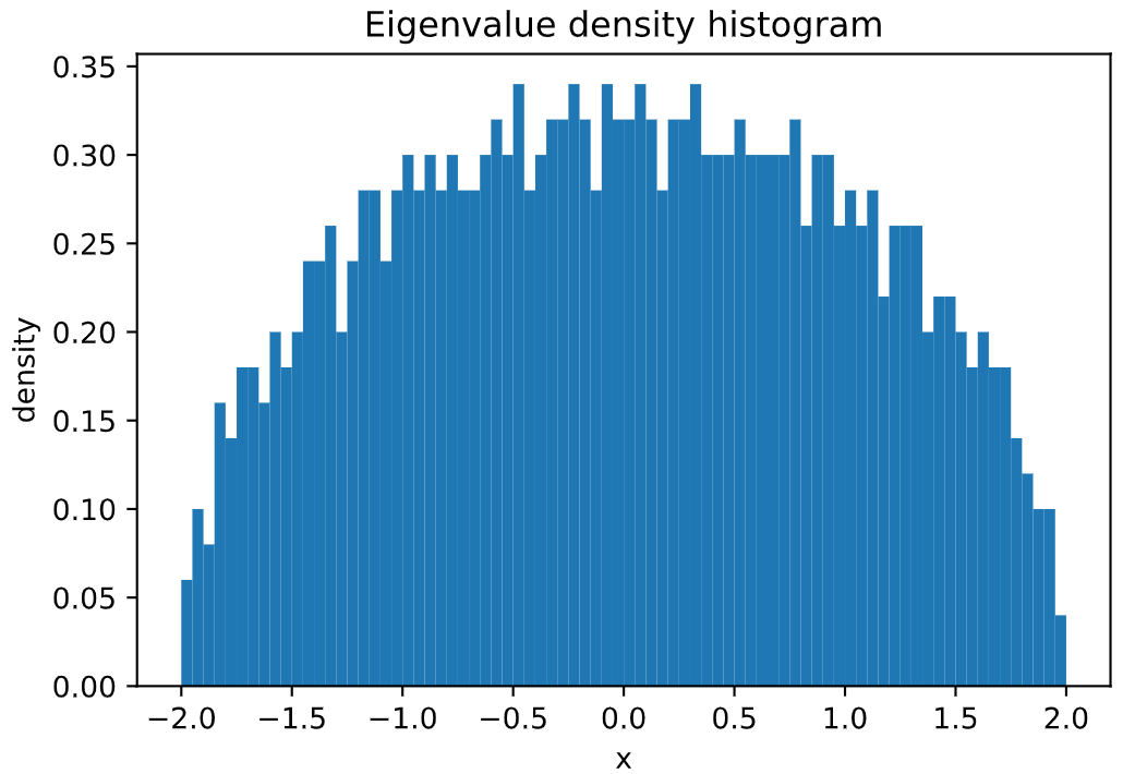
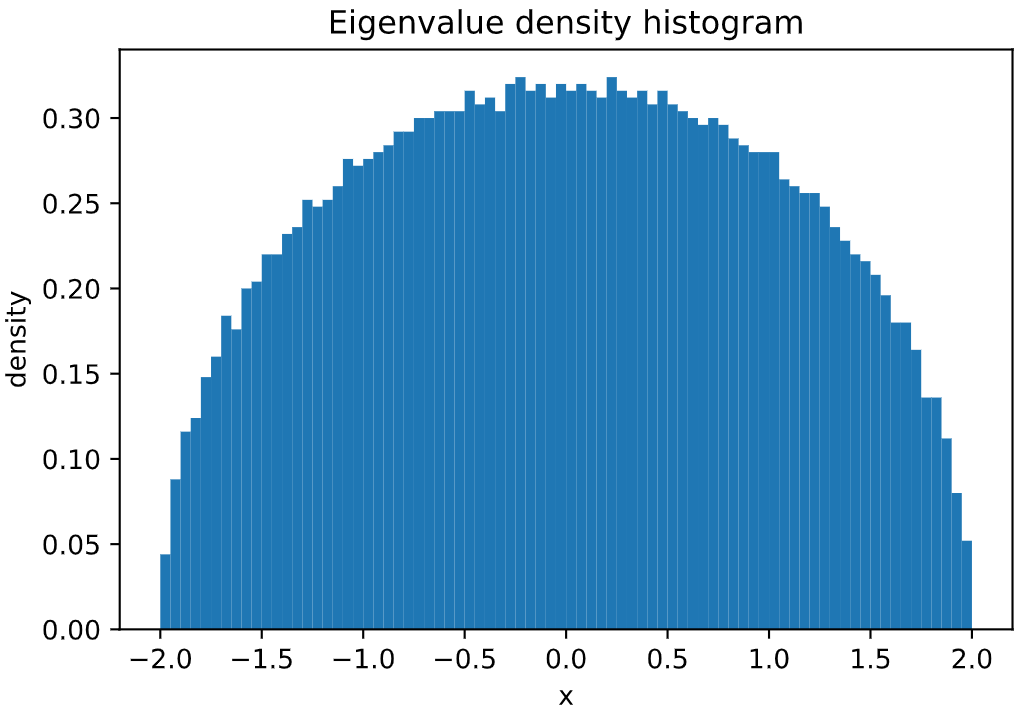
Its spectral density can be easily plotted:
```python
# sampling a GOE matrix of size 1000x1000
goe = GaussianEnsemble(beta=1, n=1000)
# plotting its spectral distribution in the interval (-2,2)
goe.plot_eigval_hist(bins=80, interval=(-2,2), density=True)
```
<!---
<img src="imgs/hist_goe.png" width=450 height=320 alt="GOE density plot">
-->
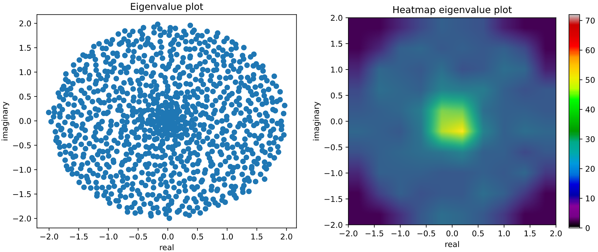
If we sample a **non-symmetric/non-hermitian** random matrix, its eigenvalues do not need to be real,
so a **2D complex histogram** has been implemented in order to study spectral density of these type
of random matrices. It would be the case, for example, of **Circular Symplectic Ensemble (CSE)**.
```python
from skrmt.ensemble.circular_ensemble import CircularEnsemble
# sampling a CSE (beta=4) matrix of size 2000x2000
cse = CircularEnsemble(beta=4, n=1000)
cse.plot_eigval_hist(bins=80)
```
<!---
<img src="imgs/hist_cse_smooth.png" width=650 height=320 alt="CSE density plot">
-->
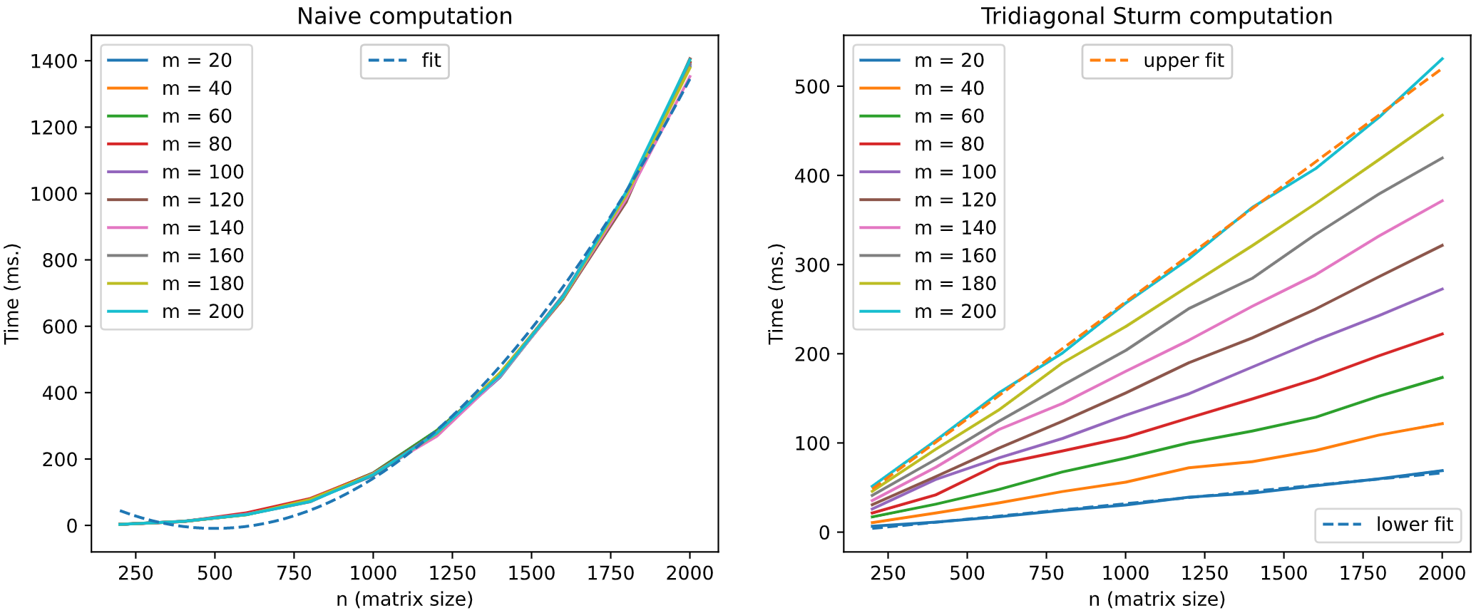
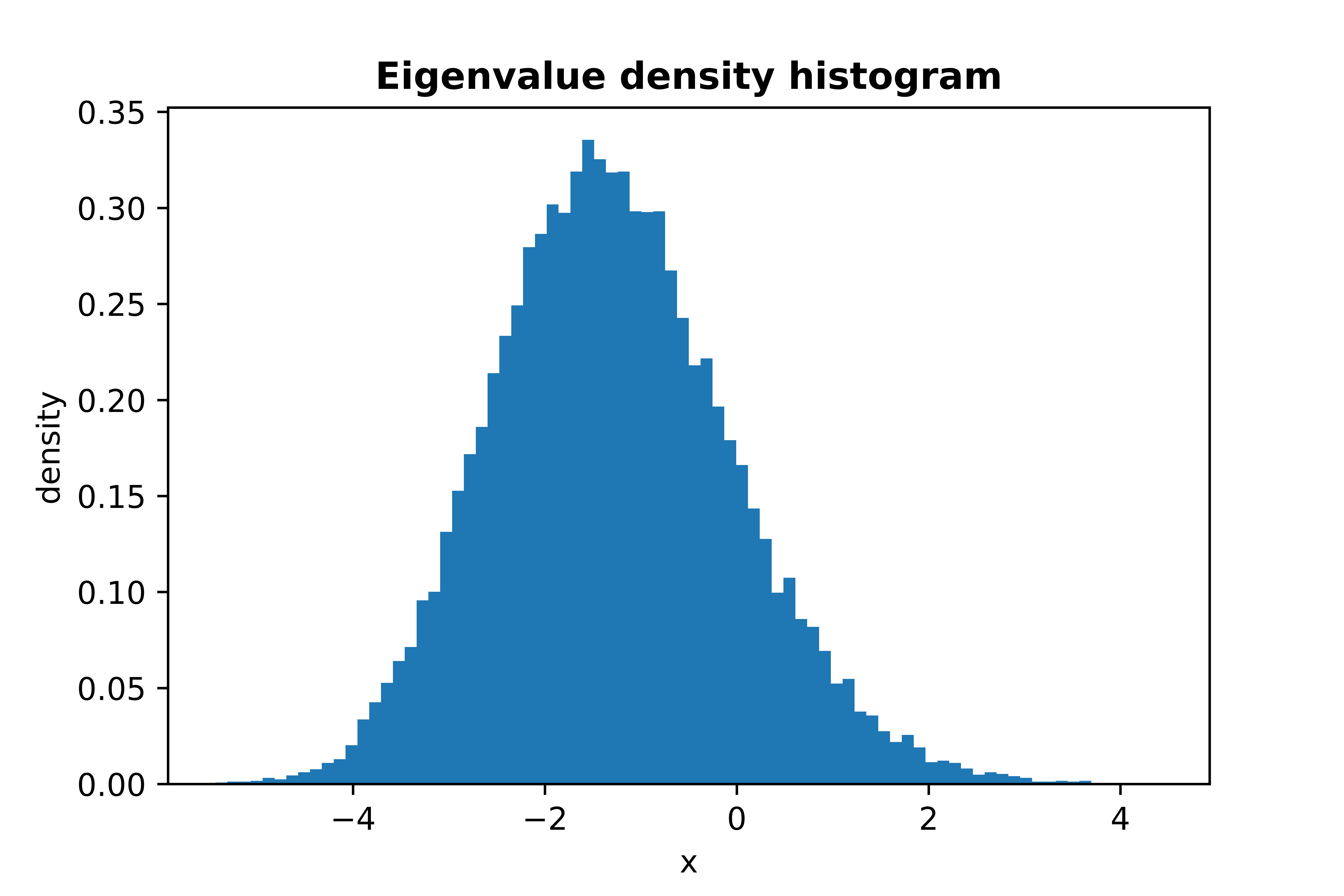
We can **boost histogram representation** using the results described by A. Edelman and I. Dumitriu
in *Matrix Models for Beta Ensembles* and by J. Albrecht, C. Chan, and A. Edelman in
*Sturm Sequences and Random Eigenvalue Distributions* (check references). Sampling certain
random matrices (**Gaussian Ensemble** and **Wishart Ensemble** matrices) in its **tridiagonal form**
we can speed up histogramming procedure. The following graphical simulation using GOE matrices
tries to illustrate it.
<!---
<img src="imgs/gauss_tridiag_sim.png" width=820 height=370 alt="Speed up by tridigonal forms">
-->
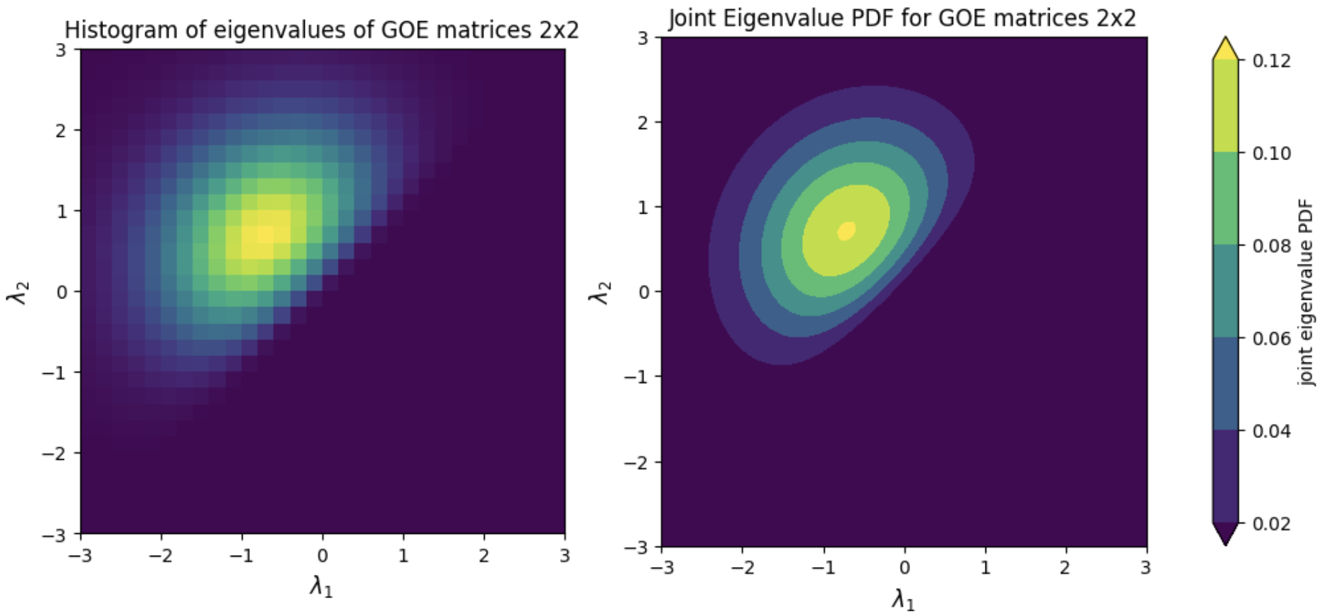
On the other hand, for all the supported ensembles, the **joint eigenvalue probability density function** can be computed by using the class method `joint_eigval_pdf(eigvals=None)`. By default, the method computes the joint eigenvalue PDF of the eigenvalues of the sampled random matrix. However, the method can be called using a pre-computed array of eigenvalues, and the joint eigenvalue PDF of these eigenvalues is returned. AS an example, we can simulate sampling and histogramming many eigenvalues of GOE random matrices of size 2x2, as well as illustrating the joint eigenvalue PDF for GOE matrices 2x2. This simulation is shown in the figure below.
<!---
<img src="imgs/goe_joint_eigval_pdf.png" width=820 height=370 alt="Joint Eigenvalue PDF for GOE">
-->
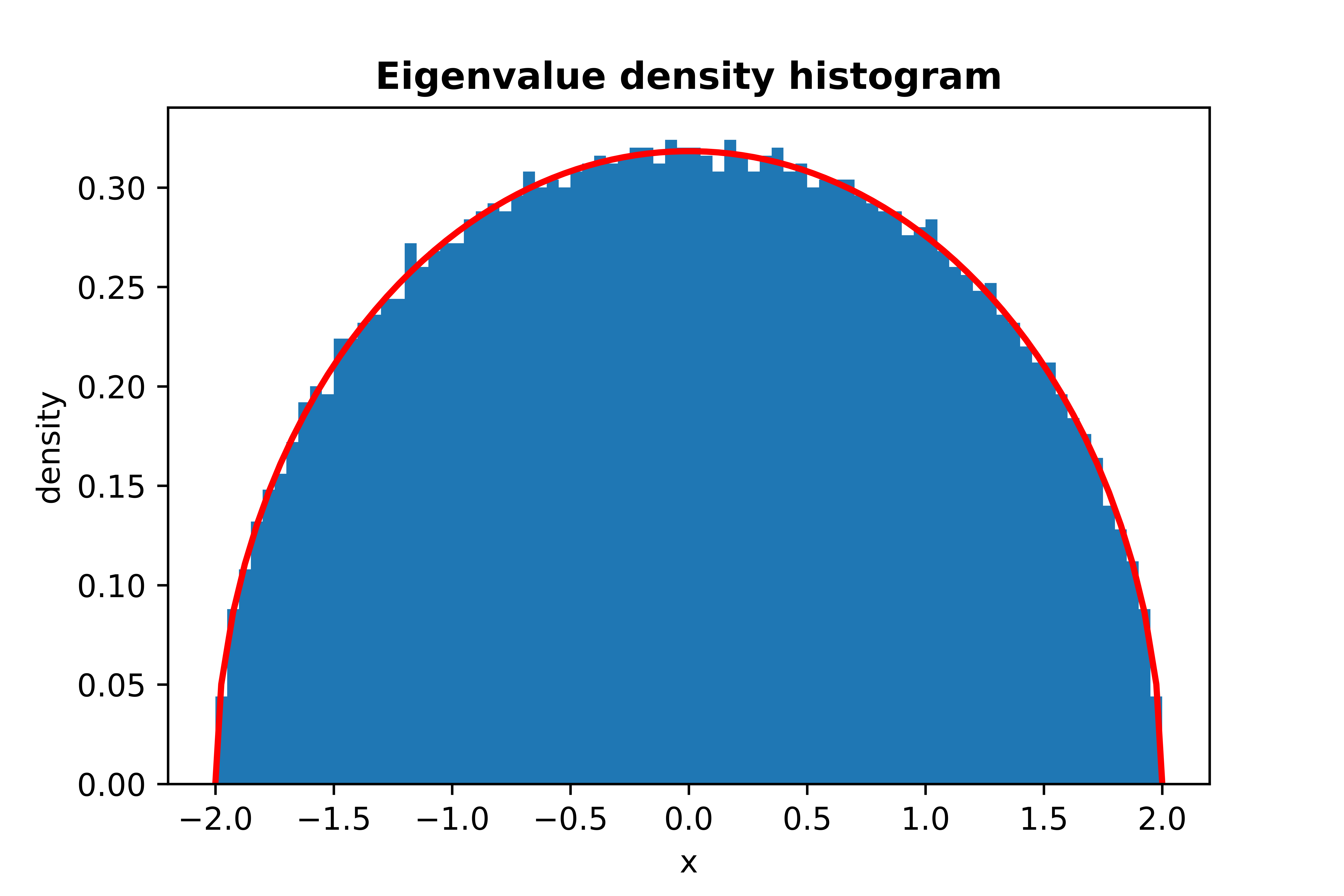
In addition, several spectral laws can be analyzed using this library, such as Wigner's Semicircle Law,
Marchenko-Pastur Law and Tracy-Widom Law. The analytical probability density function can also be plotted
by using the `plot_law_pdf=True` argument.
Plot of **Wigner's Semicircle Law**, sampling 100000 *independent* eigenvalues of a GOE matrix:
```python
from skrmt.ensemble.spectral_law import WignerSemicircleDistribution
wsd = WignerSemicircleDistribution(beta=1)
wsd.plot_empirical_pdf(sample_size=100000, bins=80, density=True)
```
<!---
<img src="imgs/scl_goe.png" width=450 height=320 alt="Wigner Semicircle Law">
-->
```python
from skrmt.ensemble.spectral_law import WignerSemicircleDistribution
wsd = WignerSemicircleDistribution(beta=1)
wsd.plot_empirical_pdf(sample_size=100000, bins=80, density=True, plot_law_pdf=True)
```
<!---
<img src="imgs/scl_goe_pdf.png" width=450 height=320 alt="Wigner Semicircle Law PDF">
-->
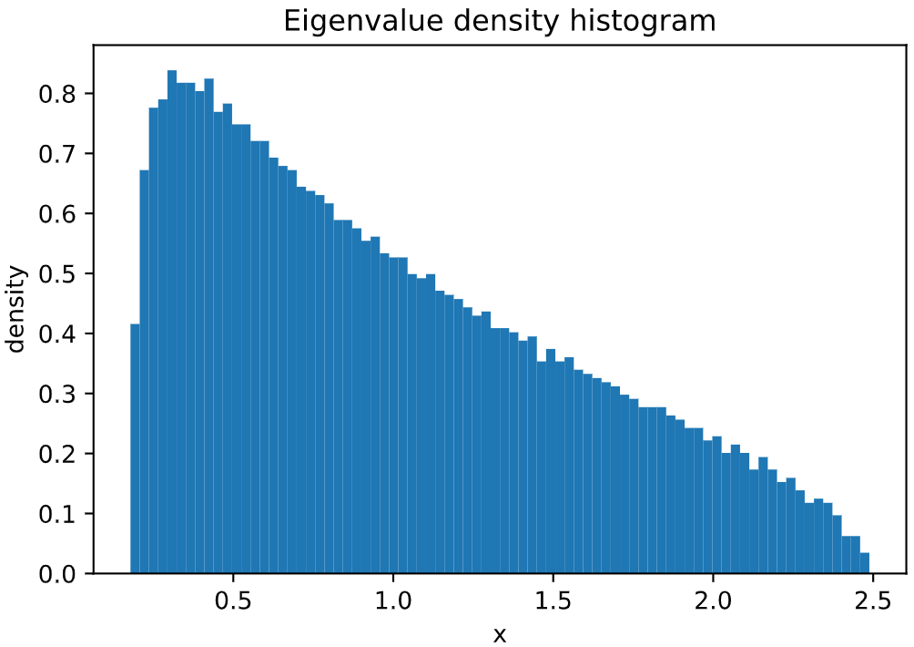
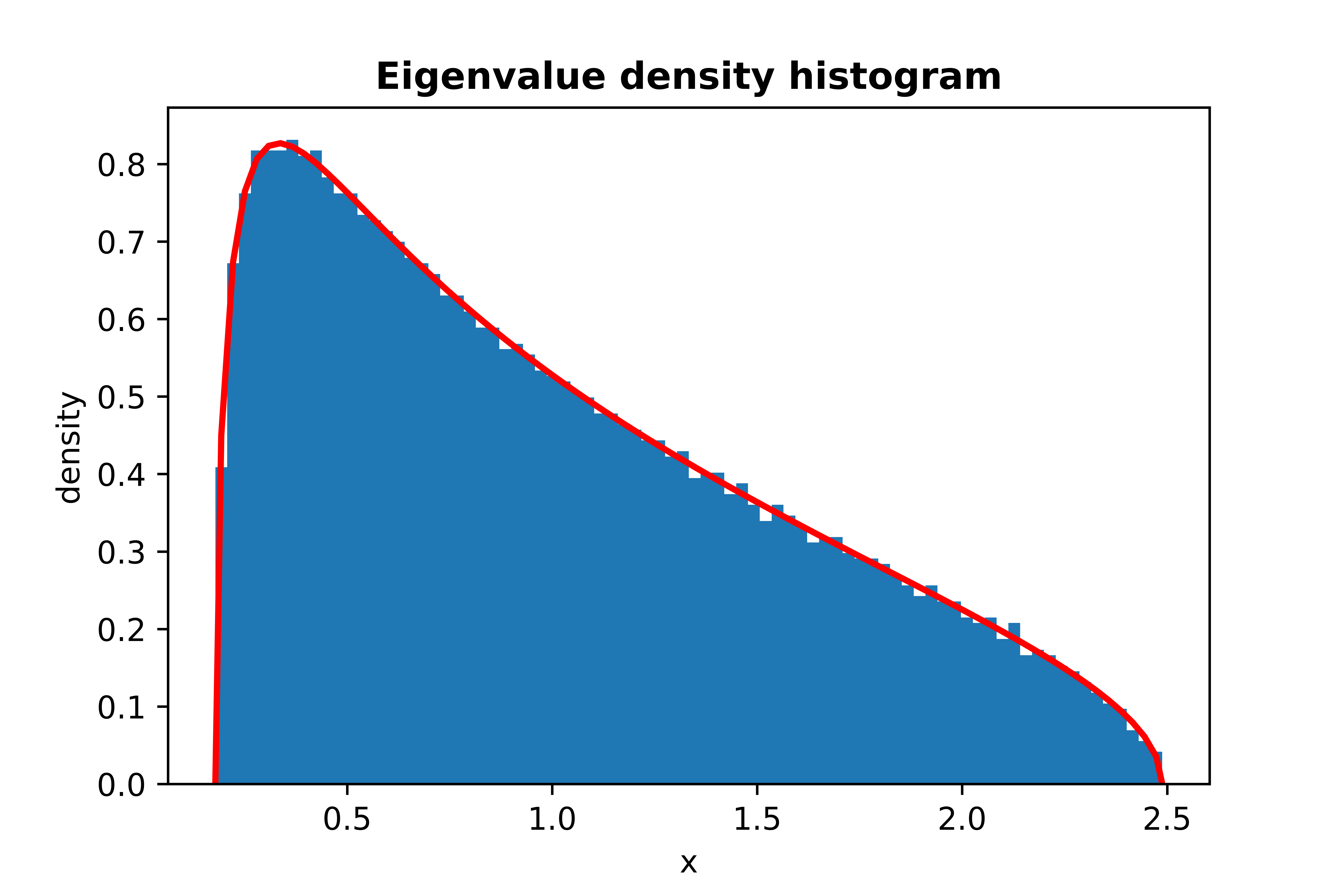
Plot of **Marchenko-Pastur Law**, sampling 100000 *independent* eigenvalues of a WRE matrix:
```python
from skrmt.ensemble.spectral_law import MarchenkoPasturDistribution
mpd = MarchenkoPasturDistribution(beta=1, ratio=1/3)
mpd.plot_empirical_pdf(sample_size=100000, bins=80, density=True)
```
<!---
<img src="imgs/mpl_wre.png" width=450 height=320 alt="Marchenko-Pastur Law">
-->
```python
from skrmt.ensemble.spectral_law import MarchenkoPasturDistribution
mpd = MarchenkoPasturDistribution(beta=1, ratio=1/3)
mpd.plot_empirical_pdf(sample_size=100000, bins=80, density=True, plot_law_pdf=True)
```
<!---
<img src="imgs/mpl_wre_pdf.png" width=450 height=320 alt="Marchenko-Pastur Law PDF">
-->
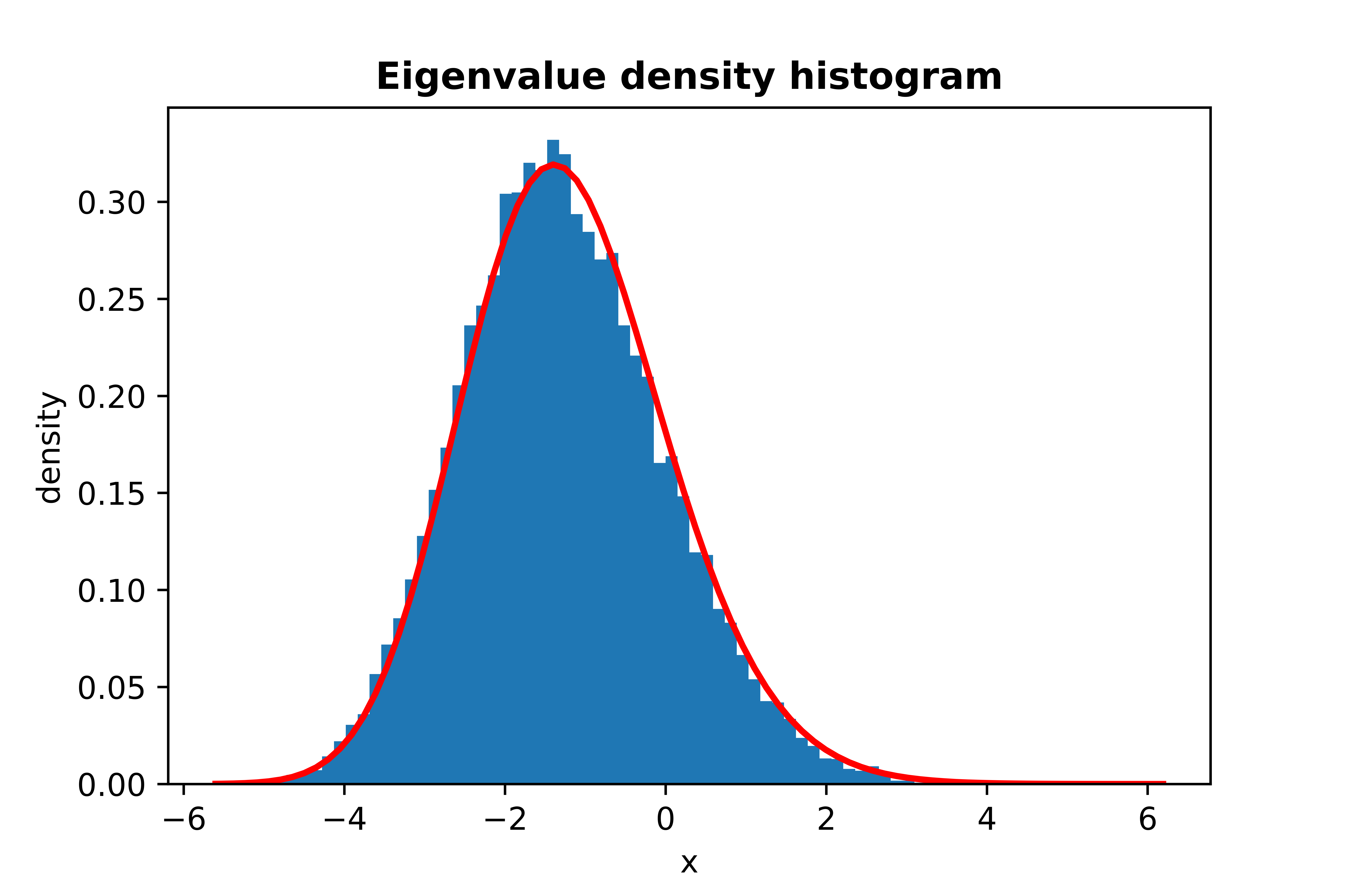
Plot of **Tracy-Widom Law**, sampling 30000 maximum eigenvalues of GOE matrices:
```python
from skrmt.ensemble.spectral_law import TracyWidomDistribution
twd = TracyWidomDistribution(beta=1)
twd.plot_empirical_pdf(sample_size=30000, bins=80, density=True)
```
<!---
<img src="imgs/twl_goe.png" width=450 height=320 alt="Tracy-Widom Law">
-->
```python
from skrmt.ensemble.spectral_law import TracyWidomDistribution
twd = TracyWidomDistribution(beta=1)
twd.plot_empirical_pdf(sample_size=30000, bins=80, density=True, plot_law_pdf=True)
```
<!---
<img src="imgs/twl_goe_pdf.png" width=450 height=320 alt="Tracy-Widom Law PDF">
-->
The proposed package **scikit-rmt** also provides support for **computing and analyzing** the **probability density function (PDF)** and **cumulative distribution function (CDF)** of the main random matrix ensembles. In particular, the following classes are implemented in the `ensemble.spectral_law` module:
- `WignerSemicircleDistribution` in `skrmt.ensemble.spectral_law`.
- `MarchenkoPasturDistribution` in `skrmt.ensemble.spectral_law`.
- `TracyWidomDistribution` in `skrmt.ensemble.spectral_law`.
- `ManovaSpectrumDistribution` in `skrmt.ensemble.spectral_law`.
For example, `WignerSemicircleDistribution` can be used to plot the **Wigner's Semicircle Law PDF**:
```python
import numpy as np
import matplotlib.pyplot as plt
from skrmt.ensemble.spectral_law import WignerSemicircleDistribution
x1 = np.linspace(-5, 5, num=1000)
x2 = np.linspace(-10, 10, num=2000)
fig, (ax1, ax2) = plt.subplots(1, 2, figsize=(12,4))
for sigma in [0.5, 1.0, 2.0, 4.0]:
wsd = WignerSemicircleDistribution(beta=1, center=0.0, sigma=sigma)
y1 = wsd.pdf(x1)
y2 = wsd.pdf(x2)
ax1.plot(x1, y1, label=f"$\sigma$ = {sigma} (R = ${wsd.radius}$)")
ax2.plot(x2, y2, label=f"$\sigma$ = {sigma} (R = ${wsd.radius}$)")
ax1.legend()
ax1.set_xlabel("x", fontweight="bold")
ax1.set_xticks([-5, -4, -3, -2, -1, 0, 1, 2, 3, 4, 5])
ax1.set_ylabel("density", fontweight="bold")
ax2.legend()
ax2.set_xlabel("x", fontweight="bold")
ax2.set_xticks([-10, -8, -6, -4, -2, 0, 2, 4, 6, 8, 10])
ax2.set_ylabel("density", fontweight="bold")
fig.suptitle("Wigner Semicircle probability density function (PDF)", fontweight="bold")
plt.show()
```
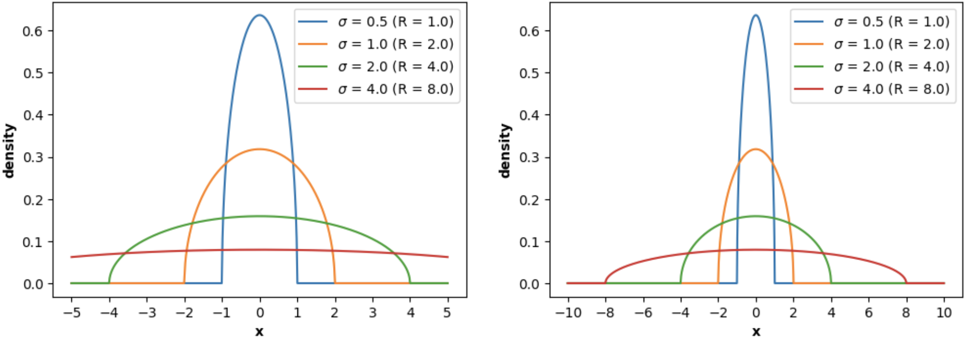
<!---
<img src="imgs/wigner_scl_pdf.png" width=450 height=320 alt="Wigner Semicircle Law PDF (Analytical)">
-->
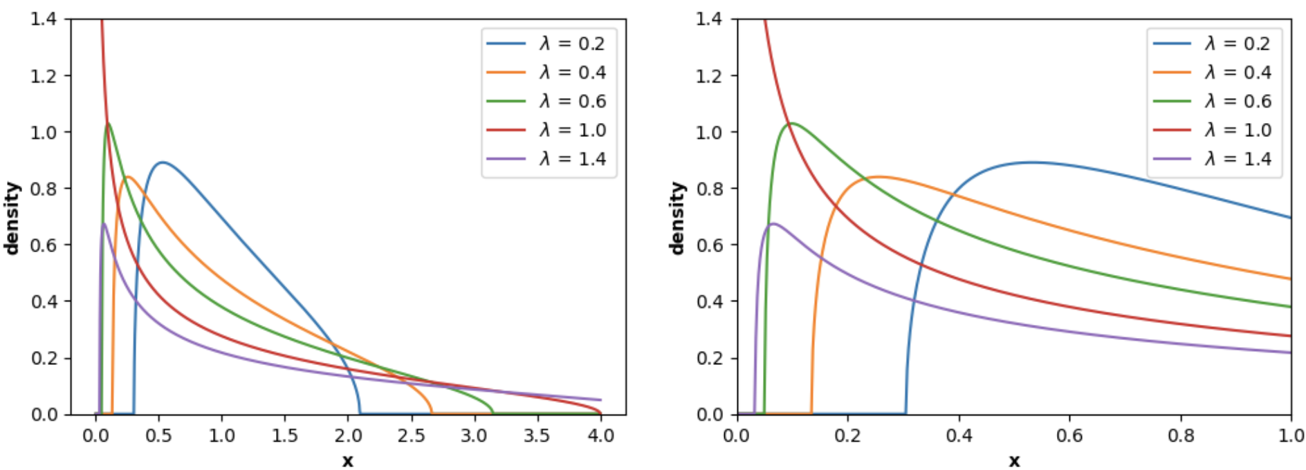
Similarly, `MarchenkoPasturDistribution` can be used to plot the **Marchenko-Pastur Law PDF**:
```python
import numpy as np
import matplotlib.pyplot as plt
from skrmt.ensemble.spectral_law import MarchenkoPasturDistribution
x1 = np.linspace(0, 4, num=1000)
x2 = np.linspace(0, 5, num=2000)
fig, (ax1, ax2) = plt.subplots(1, 2, figsize=(12,4))
for ratio in [0.2, 0.4, 0.6, 1.0, 1.4]:
mpl = MarchenkoPasturDistribution(beta=1, ratio=ratio, sigma=1.0)
y1 = mpl.pdf(x1)
y2 = mpl.pdf(x2)
ax1.plot(x1, y1, label=f"$\lambda$ = {ratio} ")
ax2.plot(x2, y2, label=f"$\lambda$ = {ratio} ")
ax1.legend()
ax1.set_ylim(0, 1.4)
ax1.set_xlabel("x", fontweight="bold")
ax1.set_ylabel("density", fontweight="bold")
ax2.legend()
ax2.set_ylim(0, 1.4)
ax2.set_xlim(0, 1)
ax2.set_xlabel("x", fontweight="bold")
ax2.set_ylabel("density", fontweight="bold")
fig.suptitle("Marchenko-Pastur probability density function (PDF)", fontweight="bold")
plt.show()
```
<!---
<img src="imgs/mpl_pdf.png" width=450 height=320 alt="Marchenko-Pastur Law PDF (Analytical)">
-->
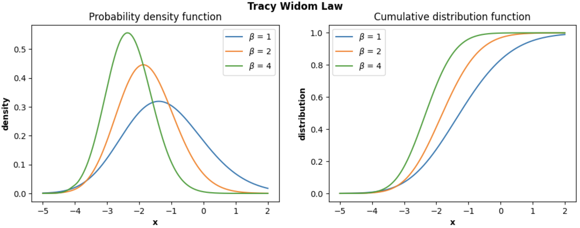
In the following example, we show how we can plot the **PDF and CDF of the Tracy-Widom distribution** using the class `TracyWidomDistribution`:
```python
import numpy as np
import matplotlib.pyplot as plt
from skrmt.ensemble.spectral_law import TracyWidomDistribution
x = np.linspace(-5, 2, num=1000)
fig, (ax1, ax2) = plt.subplots(1, 2, figsize=(12,4))
for beta in [1,2,4]:
twd = TracyWidomDistribution(beta=beta)
y_pdf = twd.pdf(x)
y_cdf = twd.cdf(x)
ax1.plot(x, y_pdf, label=f"$\\beta$ = {beta}")
ax2.plot(x, y_cdf, label=f"$\\beta$ = {beta}")
ax1.legend()
ax1.set_xlabel("x", fontweight="bold")
ax1.set_ylabel("density", fontweight="bold")
ax1.set_title("Probability density function")
ax2.legend()
ax2.set_xlabel("x", fontweight="bold")
ax2.set_ylabel("distribution", fontweight="bold")
ax2.set_title("Cumulative distribution function")
fig.suptitle("Tracy Widom Law", fontweight="bold")
plt.show()
```
<!---
<img src="imgs/twl_pdf_cdf.png" width=450 height=320 alt="Tracy-Widom Law PDF and CDF(Analytical)">
-->
The other module of this library implements **several covariance matrix estimators**:
* Sample estimator.
* Finite-sample optimal estimator (FSOpt estimator).
* Non-linear shrinkage analytical estimator (Ledoit & Wolf, 2020).
* Linear shrinkage estimator (Ledoit & Wolf, 2004).
* Empirical Bayesian estimator (Haff, 1980).
* Minimax estimator (Stain, 1982).
For certain problems, sample covariance matrix is not the best estimation for the
population covariance matrix.
The following code illustrates the usage of the estimators.
```python
from skrmt.covariance import analytical_shrinkage_estimator
# load dataset with your own/favorite function (such as pandas.read_csv)
X = load_dataset('dataset_file.data')
# get estimation
Sigma = analytical_shrinkage_estimator(X)
# ... Do something with Sigma. For example, PCA.
```
For more information or insight about the usage of the library, you can visit the official **documentation**
<https://scikit-rmt.readthedocs.io/en/latest/> or the directory [notebooks](notebooks), that contains several
*Python notebooks* with **tutorials** and plenty of **examples**.
-----------------
## License
The package is licensed under the BSD 3-Clause License. A copy of the [license](LICENSE) can be found along with the code.
-----------------
## Main references
- James Albrecht, Cy Chan, and Alan Edelman,
"Sturm Sequences and Random Eigenvalue Distributions",
*Foundations of Computational Mathematics*,
vol. 9 iss. 4 (2009), pp 461-483.
[[pdf]](http://www-math.mit.edu/~edelman/homepage/papers/sturm.pdf)
[[doi]](http://dx.doi.org/10.1007/s10208-008-9037-x)
- Ioana Dumitriu and Alan Edelman,
"Matrix Models for Beta Ensembles",
*Journal of Mathematical Physics*,
vol. 43 no. 11 (2002), pp. 5830-5547
[arXiv:math-ph/0206043](http://arxiv.org/abs/math-ph/0206043)
- Rowan Killip and Rostyslav Kozhan,
"Matrix Models and Eigenvalue Statistics for Truncations of Classical Ensembles of Random Unitary Matrices",
*Communications in Mathematical Physics*, vol. 349 (2017) pp. 991-1027.
[arxiv.org/pdf/1501.05160.pdf](http://arxiv.org/pdf/1501.05160.pdf)
- Olivier Ledoit and Michael Wolf,
"Analytical Nonlinear Shrinkage of Large-dimensional Covariance Matrices",
*Annals of Statistics*, vol. 48, no. 5 (2020) pp. 3043–3065.
[[pdf]](http://www.econ.uzh.ch/static/wp/econwp264.pdf)
- Olivier Ledoit and Michael Wolf,
"A Well-conditioned Estimator for Large-dimensional Covariance Matrices",
*Journal of Multivariate Analysis*, vol. 88 (2004) pp. 365–411.
[[pdf]](http://www.ledoit.net/ole1a.pdf)
-----------------
## Attribution
This project has been developed by Alejandro Santorum Varela (2021) as part of the final degree project
in Computer Science (Autonomous University of Madrid), supervised by Alberto Suárez González.
If you happen to use `scikit-rmt` in your work or research, please cite its GitHub repository:
A. Santorum, "scikit-rmt", https://github.com/AlejandroSantorum/scikit-rmt, 2021. GitHub repository.
The corresponding BibTex entry is
```
@misc{Santorum2021,
author = {A. Santorum},
title = {scikit-rmt},
year = {2021},
howpublished = {\url{https://github.com/AlejandroSantorum/scikit-rmt}},
note = {GitHub repository}
}
```
Raw data
{
"_id": null,
"home_page": "https://github.com/AlejandroSantorum/scikit-rmt",
"name": "scikit-rmt",
"maintainer": "",
"docs_url": null,
"requires_python": "",
"maintainer_email": "",
"keywords": "RMT,Random Matrix Theory,Ensemble,Covariance matrices",
"author": "Alejandro Santorum Varela",
"author_email": "alejandro.santorum@gmail.com",
"download_url": "https://files.pythonhosted.org/packages/f4/e8/7545634f96412a8d0aa6410935ba19fc704468b473ceb539099b67e54d47/scikit-rmt-0.10.4.tar.gz",
"platform": null,
"description": "\n\n\n[](https://pypi.org/project/scikit-rmt/)\n[](https://github.com/AlejandroSantorum/scikit-rmt/actions/workflows/tests.yaml?event=push)\n[](https://scikit-rmt.readthedocs.io/en/latest/?badge=latest)\n[](https://codecov.io/gh/AlejandroSantorum/scikit-rmt/)\n[](https://github.com/AlejandroSantorum/scikit-rmt/blob/main/LICENSE)\n[](https://pypi.org/project/scikit-rmt)\n\n\n# scikit-rmt: Random Matrix Theory Python package\n\nRandom Matrix Theory, or RMT, is the field of Statistics that analyses\nmatrices that their entries are random variables.\n\nThis package offers classes, methods and functions to give support to RMT\nin Python. Includes a wide range of utils to work with different random\nmatrix ensembles, random matrix spectral laws and estimation of covariance\nmatrices. See documentation or visit the <https://github.com/AlejandroSantorum/scikit-rmt>\nof the project for further information on the features included in the package.\n\n-----------------\n## Documentation\n\nThe documentation is available at <https://scikit-rmt.readthedocs.io/en/latest/>,\nwhich includes detailed information of the different modules, classes and methods of\nthe package, along with several examples showing different funcionalities.\n\n-----------------\n## Installation\n\nUsing a virtual environment is recommended to minimize the chance of conflicts.\nHowever, the global installation _should_ work properly as well.\n\n### Local installation using `venv` (recommended)\n\nNavigate to your project directory.\n```bash\ncd MyProject\n```\n\nCreate a virtual environment (you can change the name \"env\").\n```bash\npython3 -m venv env\n```\n\nActivate the environment \"env\".\n```bash\nsource env/bin/activate\n```\n\nInstall using `pip`.\n```bash\npip install scikit-rmt\n```\nYou may need to use `pip3`.\n```bash\npip3 install scikit-rmt\n```\n\n### Global installation\nJust install it using `pip` or `pip3`.\n```bash\npip install scikit-rmt\n```\n\n### Requirements\n*scikit-rmt* depends on the following packages:\n* [numpy](https://github.com/numpy/numpy) - The fundamental package for scientific computing with Python\n* [matplotlib](https://github.com/matplotlib/matplotlib) - Plotting with Python\n* [scipy](https://github.com/scipy/scipy) - Scientific computation in Python\n\nCheck the pinned versions in the [requirements.txt](requirements.txt) file.\n\n----------------\n## Main features\n*scikit-rmt* provides support to analyze, study and simulate Random Matrix Theory properties and results:\n* **Sampling** of the following random matrix ensembles:\n * Gaussian Ensemble (GOE, GUE and GSE; for beta=1, 2 and 4 respectively): class `GaussianEnsemble`.\n * Wishart Ensemble (WRE, WCE and WQE; for beta=1, 2 and 4 respectively): class `WishartEnsemble`.\n * Manova Ensemble (MRE, MCE and MQE; for beta=1, 2 and 4 respectively): class `ManovaEnsemble`.\n * Circular Ensemble (COE, CUE, CSE; for beta=1, 2 and 4 respectively): class `CircularEnsemble`.\n* **Eigenvalue computation** for the previous ensembles using the class method `eigvals`.\n* Computation of the **joint eigenvalue probability density function** given the random matrix eigenvalues, using the class method `joint_eigval_pdf`.\n* Computation of the **empirical spectral histogram** by executing the class method `eigval_hist`.\n* **Plotting of the empirical spectral histogram** using the class method `plot_eigval_hist`.\n* Computation and plotting of the following **spectral laws** (`spectral_law` sub-module), including the calculation and plotting of the corresponding probability density functions (PDFs) and cumulative distribution functions (CDFs):\n * **Wigner Semicircle law**: describes the limiting distribution of the eigenvalues of Wigner matrices (in particular, random matrices from the Gaussian Ensemble). Implemented by class `WignerSemicircleDistribution`.\n * **Tracy-Widom law**: describes the limiting distribution of the largest eigenvalue of Wigner matrices (in particular, random matrices from the Gaussian Ensemble). Implemented by class `TracyWidomDistribution`.\n * **Marchenko-Pastur law**: describes the limiting distribution of the eigenvalues of Wishart matrices (random matrices from the Wishart Ensemble). Implemented by class `MarchenkoPasturDistribution`.\n * **Manova Spectrum law**: introduced and proved by K. W. Wachter (1980), it describes the limiting distribution of the eigenvalues of Manova matrices (random matrices from the Manova Ensemble). Implemented by class `ManovaSpectrumDistribution`.\n* **Covariance matrix estimation** using different matrix smoothing and estimation methods (`covariance` module).\n * Estimation of sample covariance matrix using `sample_estimator` function.\n * Finite-sample Optimal (FSOpt) estimator by `fsopt_estimator` function.\n * Empirical Bayesian estimator by `empirical_bayesian_estimator` function. Haff in *\"Estimation of a covariance matrix under Stein\u2019s loss\"* (1985).\n * Minimax estimator by `minimax_estimator` function \n * Linear shrinkage estimator by `linear_shrinkage_estimator` function. Ledoit and Wolf in *\"A well-conditioned estimator for large-dimensional covariance matrices\"* (2004).\n * Analytical shrinkage estimator by `analytical_shrinkage_estimator` function. Ledoit and Wolf in *\"Analytical nonlinear shrinkage of large-dimensional covariance matrices\"* (2020).\n\n\n-----------------\n## A brief tutorial\n\nFirst of all, several random matrix ensembles can be sampled: **Gaussian Ensembles**, **Wishart Ensembles**,\n**Manova Ensembles** and **Circular Ensembles**. As an example, the following code shows how to sample\na **Gaussian Orthogonal Ensemble (GOE)** random matrix.\n\n```python\nfrom skrmt.ensemble.gaussian_ensemble import GaussianEnsemble\n# sampling a GOE (beta=1) matrix of size 3x3\ngoe = GaussianEnsemble(beta=1, n=3)\nprint(goe.matrix)\n```\n```bash\n[[ 0.34574696 -0.10802385 0.38245343]\n [-0.10802385 -0.60113963 0.28624612]\n [ 0.38245343 0.28624612 -0.96503739]]\n```\nIts spectral density can be easily plotted:\n```python\n# sampling a GOE matrix of size 1000x1000\ngoe = GaussianEnsemble(beta=1, n=1000)\n# plotting its spectral distribution in the interval (-2,2)\ngoe.plot_eigval_hist(bins=80, interval=(-2,2), density=True)\n```\n\n<!---\n<img src=\"imgs/hist_goe.png\" width=450 height=320 alt=\"GOE density plot\">\n-->\n\nIf we sample a **non-symmetric/non-hermitian** random matrix, its eigenvalues do not need to be real,\nso a **2D complex histogram** has been implemented in order to study spectral density of these type\nof random matrices. It would be the case, for example, of **Circular Symplectic Ensemble (CSE)**.\n\n```python\nfrom skrmt.ensemble.circular_ensemble import CircularEnsemble\n\n# sampling a CSE (beta=4) matrix of size 2000x2000\ncse = CircularEnsemble(beta=4, n=1000)\ncse.plot_eigval_hist(bins=80)\n```\n\n<!---\n<img src=\"imgs/hist_cse_smooth.png\" width=650 height=320 alt=\"CSE density plot\">\n-->\n\nWe can **boost histogram representation** using the results described by A. Edelman and I. Dumitriu\nin *Matrix Models for Beta Ensembles* and by J. Albrecht, C. Chan, and A. Edelman in\n*Sturm Sequences and Random Eigenvalue Distributions* (check references). Sampling certain\nrandom matrices (**Gaussian Ensemble** and **Wishart Ensemble** matrices) in its **tridiagonal form**\nwe can speed up histogramming procedure. The following graphical simulation using GOE matrices\ntries to illustrate it.\n\n<!---\n<img src=\"imgs/gauss_tridiag_sim.png\" width=820 height=370 alt=\"Speed up by tridigonal forms\">\n-->\n\nOn the other hand, for all the supported ensembles, the **joint eigenvalue probability density function** can be computed by using the class method `joint_eigval_pdf(eigvals=None)`. By default, the method computes the joint eigenvalue PDF of the eigenvalues of the sampled random matrix. However, the method can be called using a pre-computed array of eigenvalues, and the joint eigenvalue PDF of these eigenvalues is returned. AS an example, we can simulate sampling and histogramming many eigenvalues of GOE random matrices of size 2x2, as well as illustrating the joint eigenvalue PDF for GOE matrices 2x2. This simulation is shown in the figure below.\n\n<!---\n<img src=\"imgs/goe_joint_eigval_pdf.png\" width=820 height=370 alt=\"Joint Eigenvalue PDF for GOE\">\n-->\n\nIn addition, several spectral laws can be analyzed using this library, such as Wigner's Semicircle Law,\nMarchenko-Pastur Law and Tracy-Widom Law. The analytical probability density function can also be plotted\nby using the `plot_law_pdf=True` argument.\n\nPlot of **Wigner's Semicircle Law**, sampling 100000 *independent* eigenvalues of a GOE matrix:\n```python\nfrom skrmt.ensemble.spectral_law import WignerSemicircleDistribution\n\nwsd = WignerSemicircleDistribution(beta=1)\nwsd.plot_empirical_pdf(sample_size=100000, bins=80, density=True)\n```\n\n<!---\n<img src=\"imgs/scl_goe.png\" width=450 height=320 alt=\"Wigner Semicircle Law\">\n-->\n\n```python\nfrom skrmt.ensemble.spectral_law import WignerSemicircleDistribution\n\nwsd = WignerSemicircleDistribution(beta=1)\nwsd.plot_empirical_pdf(sample_size=100000, bins=80, density=True, plot_law_pdf=True)\n```\n\n<!---\n<img src=\"imgs/scl_goe_pdf.png\" width=450 height=320 alt=\"Wigner Semicircle Law PDF\">\n-->\n\nPlot of **Marchenko-Pastur Law**, sampling 100000 *independent* eigenvalues of a WRE matrix:\n```python\nfrom skrmt.ensemble.spectral_law import MarchenkoPasturDistribution\n\nmpd = MarchenkoPasturDistribution(beta=1, ratio=1/3)\nmpd.plot_empirical_pdf(sample_size=100000, bins=80, density=True)\n```\n\n<!---\n<img src=\"imgs/mpl_wre.png\" width=450 height=320 alt=\"Marchenko-Pastur Law\">\n-->\n\n```python\nfrom skrmt.ensemble.spectral_law import MarchenkoPasturDistribution\n\nmpd = MarchenkoPasturDistribution(beta=1, ratio=1/3)\nmpd.plot_empirical_pdf(sample_size=100000, bins=80, density=True, plot_law_pdf=True)\n```\n\n<!---\n<img src=\"imgs/mpl_wre_pdf.png\" width=450 height=320 alt=\"Marchenko-Pastur Law PDF\">\n-->\n\nPlot of **Tracy-Widom Law**, sampling 30000 maximum eigenvalues of GOE matrices:\n```python\nfrom skrmt.ensemble.spectral_law import TracyWidomDistribution\n\ntwd = TracyWidomDistribution(beta=1)\ntwd.plot_empirical_pdf(sample_size=30000, bins=80, density=True)\n```\n\n<!---\n<img src=\"imgs/twl_goe.png\" width=450 height=320 alt=\"Tracy-Widom Law\">\n-->\n\n```python\nfrom skrmt.ensemble.spectral_law import TracyWidomDistribution\n\ntwd = TracyWidomDistribution(beta=1)\ntwd.plot_empirical_pdf(sample_size=30000, bins=80, density=True, plot_law_pdf=True)\n```\n\n<!---\n<img src=\"imgs/twl_goe_pdf.png\" width=450 height=320 alt=\"Tracy-Widom Law PDF\">\n-->\n\nThe proposed package **scikit-rmt** also provides support for **computing and analyzing** the **probability density function (PDF)** and **cumulative distribution function (CDF)** of the main random matrix ensembles. In particular, the following classes are implemented in the `ensemble.spectral_law` module:\n- `WignerSemicircleDistribution` in `skrmt.ensemble.spectral_law`.\n- `MarchenkoPasturDistribution` in `skrmt.ensemble.spectral_law`.\n- `TracyWidomDistribution` in `skrmt.ensemble.spectral_law`.\n- `ManovaSpectrumDistribution` in `skrmt.ensemble.spectral_law`.\n\nFor example, `WignerSemicircleDistribution` can be used to plot the **Wigner's Semicircle Law PDF**:\n```python\nimport numpy as np\nimport matplotlib.pyplot as plt\nfrom skrmt.ensemble.spectral_law import WignerSemicircleDistribution\n\nx1 = np.linspace(-5, 5, num=1000)\nx2 = np.linspace(-10, 10, num=2000)\n\nfig, (ax1, ax2) = plt.subplots(1, 2, figsize=(12,4))\n\nfor sigma in [0.5, 1.0, 2.0, 4.0]:\n wsd = WignerSemicircleDistribution(beta=1, center=0.0, sigma=sigma)\n\n y1 = wsd.pdf(x1)\n y2 = wsd.pdf(x2)\n\n ax1.plot(x1, y1, label=f\"$\\sigma$ = {sigma} (R = ${wsd.radius}$)\")\n ax2.plot(x2, y2, label=f\"$\\sigma$ = {sigma} (R = ${wsd.radius}$)\")\n\nax1.legend()\nax1.set_xlabel(\"x\", fontweight=\"bold\")\nax1.set_xticks([-5, -4, -3, -2, -1, 0, 1, 2, 3, 4, 5])\nax1.set_ylabel(\"density\", fontweight=\"bold\")\n\nax2.legend()\nax2.set_xlabel(\"x\", fontweight=\"bold\")\nax2.set_xticks([-10, -8, -6, -4, -2, 0, 2, 4, 6, 8, 10])\nax2.set_ylabel(\"density\", fontweight=\"bold\")\n\nfig.suptitle(\"Wigner Semicircle probability density function (PDF)\", fontweight=\"bold\")\nplt.show()\n```\n\n<!---\n<img src=\"imgs/wigner_scl_pdf.png\" width=450 height=320 alt=\"Wigner Semicircle Law PDF (Analytical)\">\n-->\n\nSimilarly, `MarchenkoPasturDistribution` can be used to plot the **Marchenko-Pastur Law PDF**:\n```python\nimport numpy as np\nimport matplotlib.pyplot as plt\nfrom skrmt.ensemble.spectral_law import MarchenkoPasturDistribution\n\nx1 = np.linspace(0, 4, num=1000)\nx2 = np.linspace(0, 5, num=2000)\n\nfig, (ax1, ax2) = plt.subplots(1, 2, figsize=(12,4))\n\nfor ratio in [0.2, 0.4, 0.6, 1.0, 1.4]:\n mpl = MarchenkoPasturDistribution(beta=1, ratio=ratio, sigma=1.0)\n\n y1 = mpl.pdf(x1)\n y2 = mpl.pdf(x2)\n\n ax1.plot(x1, y1, label=f\"$\\lambda$ = {ratio} \")\n ax2.plot(x2, y2, label=f\"$\\lambda$ = {ratio} \")\n\nax1.legend()\nax1.set_ylim(0, 1.4)\nax1.set_xlabel(\"x\", fontweight=\"bold\")\nax1.set_ylabel(\"density\", fontweight=\"bold\")\n\nax2.legend()\nax2.set_ylim(0, 1.4)\nax2.set_xlim(0, 1)\nax2.set_xlabel(\"x\", fontweight=\"bold\")\nax2.set_ylabel(\"density\", fontweight=\"bold\")\n\nfig.suptitle(\"Marchenko-Pastur probability density function (PDF)\", fontweight=\"bold\")\nplt.show()\n```\n\n<!---\n<img src=\"imgs/mpl_pdf.png\" width=450 height=320 alt=\"Marchenko-Pastur Law PDF (Analytical)\">\n-->\n\nIn the following example, we show how we can plot the **PDF and CDF of the Tracy-Widom distribution** using the class `TracyWidomDistribution`:\n```python\nimport numpy as np\nimport matplotlib.pyplot as plt\nfrom skrmt.ensemble.spectral_law import TracyWidomDistribution\n\nx = np.linspace(-5, 2, num=1000)\n\nfig, (ax1, ax2) = plt.subplots(1, 2, figsize=(12,4))\n\nfor beta in [1,2,4]:\n twd = TracyWidomDistribution(beta=beta)\n\n y_pdf = twd.pdf(x)\n y_cdf = twd.cdf(x)\n\n ax1.plot(x, y_pdf, label=f\"$\\\\beta$ = {beta}\")\n ax2.plot(x, y_cdf, label=f\"$\\\\beta$ = {beta}\")\n\nax1.legend()\nax1.set_xlabel(\"x\", fontweight=\"bold\")\nax1.set_ylabel(\"density\", fontweight=\"bold\")\nax1.set_title(\"Probability density function\")\n\nax2.legend()\nax2.set_xlabel(\"x\", fontweight=\"bold\")\nax2.set_ylabel(\"distribution\", fontweight=\"bold\")\nax2.set_title(\"Cumulative distribution function\")\n\nfig.suptitle(\"Tracy Widom Law\", fontweight=\"bold\")\nplt.show()\n```\n\n<!---\n<img src=\"imgs/twl_pdf_cdf.png\" width=450 height=320 alt=\"Tracy-Widom Law PDF and CDF(Analytical)\">\n-->\n\n\nThe other module of this library implements **several covariance matrix estimators**:\n* Sample estimator.\n* Finite-sample optimal estimator (FSOpt estimator).\n* Non-linear shrinkage analytical estimator (Ledoit & Wolf, 2020).\n* Linear shrinkage estimator (Ledoit & Wolf, 2004).\n* Empirical Bayesian estimator (Haff, 1980).\n* Minimax estimator (Stain, 1982).\n\nFor certain problems, sample covariance matrix is not the best estimation for the\npopulation covariance matrix.\n\nThe following code illustrates the usage of the estimators.\n```python\nfrom skrmt.covariance import analytical_shrinkage_estimator\n\n# load dataset with your own/favorite function (such as pandas.read_csv)\nX = load_dataset('dataset_file.data')\n\n# get estimation\nSigma = analytical_shrinkage_estimator(X)\n\n# ... Do something with Sigma. For example, PCA.\n```\n\nFor more information or insight about the usage of the library, you can visit the official **documentation** \n<https://scikit-rmt.readthedocs.io/en/latest/> or the directory [notebooks](notebooks), that contains several\n*Python notebooks* with **tutorials** and plenty of **examples**.\n\n-----------------\n## License\nThe package is licensed under the BSD 3-Clause License. A copy of the [license](LICENSE) can be found along with the code.\n\n-----------------\n## Main references\n\n- James Albrecht, Cy Chan, and Alan Edelman,\n \"Sturm Sequences and Random Eigenvalue Distributions\",\n *Foundations of Computational Mathematics*,\n vol. 9 iss. 4 (2009), pp 461-483.\n [[pdf]](http://www-math.mit.edu/~edelman/homepage/papers/sturm.pdf)\n [[doi]](http://dx.doi.org/10.1007/s10208-008-9037-x)\n\n- Ioana Dumitriu and Alan Edelman,\n \"Matrix Models for Beta Ensembles\",\n *Journal of Mathematical Physics*,\n vol. 43 no. 11 (2002), pp. 5830-5547\n [arXiv:math-ph/0206043](http://arxiv.org/abs/math-ph/0206043)\n\n- Rowan Killip and Rostyslav Kozhan,\n \"Matrix Models and Eigenvalue Statistics for Truncations of Classical Ensembles of Random Unitary Matrices\",\n *Communications in Mathematical Physics*, vol. 349 (2017) pp. 991-1027.\n [arxiv.org/pdf/1501.05160.pdf](http://arxiv.org/pdf/1501.05160.pdf)\n\n- Olivier Ledoit and Michael Wolf,\n \"Analytical Nonlinear Shrinkage of Large-dimensional Covariance Matrices\",\n *Annals of Statistics*, vol. 48, no. 5 (2020) pp. 3043\u20133065.\n [[pdf]](http://www.econ.uzh.ch/static/wp/econwp264.pdf)\n\n- Olivier Ledoit and Michael Wolf,\n \"A Well-conditioned Estimator for Large-dimensional Covariance Matrices\",\n *Journal of Multivariate Analysis*, vol. 88 (2004) pp. 365\u2013411.\n [[pdf]](http://www.ledoit.net/ole1a.pdf)\n\n-----------------\n## Attribution\nThis project has been developed by Alejandro Santorum Varela (2021) as part of the final degree project\nin Computer Science (Autonomous University of Madrid), supervised by Alberto Su\u00e1rez Gonz\u00e1lez.\n\nIf you happen to use `scikit-rmt` in your work or research, please cite its GitHub repository:\n\nA. Santorum, \"scikit-rmt\", https://github.com/AlejandroSantorum/scikit-rmt, 2021. GitHub repository.\n\nThe corresponding BibTex entry is\n```\n@misc{Santorum2021,\n author = {A. Santorum},\n title = {scikit-rmt},\n year = {2021},\n howpublished = {\\url{https://github.com/AlejandroSantorum/scikit-rmt}},\n note = {GitHub repository}\n}\n```",
"bugtrack_url": null,
"license": "BSD",
"summary": "Random Matrix Theory Python package",
"version": "0.10.4",
"project_urls": {
"Download": "https://github.com/AlejandroSantorum/scikit-rmt/archive/refs/tags/v0.10.4.tar.gz",
"Homepage": "https://github.com/AlejandroSantorum/scikit-rmt"
},
"split_keywords": [
"rmt",
"random matrix theory",
"ensemble",
"covariance matrices"
],
"urls": [
{
"comment_text": "",
"digests": {
"blake2b_256": "f4e87545634f96412a8d0aa6410935ba19fc704468b473ceb539099b67e54d47",
"md5": "a03bd0637e569c9021ce53630b1996e0",
"sha256": "aa3ceca4daa26ef95f1ef9d16af0235f91ab72142e19c60f4c4bf8c6f810a12d"
},
"downloads": -1,
"filename": "scikit-rmt-0.10.4.tar.gz",
"has_sig": false,
"md5_digest": "a03bd0637e569c9021ce53630b1996e0",
"packagetype": "sdist",
"python_version": "source",
"requires_python": null,
"size": 82354,
"upload_time": "2023-09-18T18:56:13",
"upload_time_iso_8601": "2023-09-18T18:56:13.775604Z",
"url": "https://files.pythonhosted.org/packages/f4/e8/7545634f96412a8d0aa6410935ba19fc704468b473ceb539099b67e54d47/scikit-rmt-0.10.4.tar.gz",
"yanked": false,
"yanked_reason": null
}
],
"upload_time": "2023-09-18 18:56:13",
"github": true,
"gitlab": false,
"bitbucket": false,
"codeberg": false,
"github_user": "AlejandroSantorum",
"github_project": "scikit-rmt",
"travis_ci": false,
"coveralls": true,
"github_actions": true,
"requirements": [],
"lcname": "scikit-rmt"
}


