# [scikit-opt](https://github.com/guofei9987/scikit-opt)
[](https://pypi.org/project/scikit-opt/)
[](https://travis-ci.com/guofei9987/scikit-opt)
[](https://codecov.io/gh/guofei9987/scikit-opt)
[](https://github.com/guofei9987/scikit-opt/blob/master/LICENSE)


[](https://github.com/guofei9987/scikit-opt/fork)
[](https://pepy.tech/project/scikit-opt)
[](https://github.com/guofei9987/scikit-opt/discussions)
Swarm Intelligence in Python
(Genetic Algorithm, Particle Swarm Optimization, Simulated Annealing, Ant Colony Algorithm, Immune Algorithm,Artificial Fish Swarm Algorithm in Python)
- **Documentation:** [https://scikit-opt.github.io/scikit-opt/#/en/](https://scikit-opt.github.io/scikit-opt/#/en/)
- **文档:** [https://scikit-opt.github.io/scikit-opt/#/zh/](https://scikit-opt.github.io/scikit-opt/#/zh/)
- **Source code:** [https://github.com/guofei9987/scikit-opt](https://github.com/guofei9987/scikit-opt)
- **Help us improve scikit-opt** [https://www.wjx.cn/jq/50964691.aspx](https://www.wjx.cn/jq/50964691.aspx)
# install
```bash
pip install scikit-opt
```
For the current developer version:
```bach
git clone git@github.com:guofei9987/scikit-opt.git
cd scikit-opt
pip install .
```
# Features
## Feature1: UDF
**UDF** (user defined function) is available now!
For example, you just worked out a new type of `selection` function.
Now, your `selection` function is like this:
-> Demo code: [examples/demo_ga_udf.py#s1](https://github.com/guofei9987/scikit-opt/blob/master/examples/demo_ga_udf.py#L1)
```python
# step1: define your own operator:
def selection_tournament(algorithm, tourn_size):
FitV = algorithm.FitV
sel_index = []
for i in range(algorithm.size_pop):
aspirants_index = np.random.choice(range(algorithm.size_pop), size=tourn_size)
sel_index.append(max(aspirants_index, key=lambda i: FitV[i]))
algorithm.Chrom = algorithm.Chrom[sel_index, :] # next generation
return algorithm.Chrom
```
Import and build ga
-> Demo code: [examples/demo_ga_udf.py#s2](https://github.com/guofei9987/scikit-opt/blob/master/examples/demo_ga_udf.py#L12)
```python
import numpy as np
from sko.GA import GA, GA_TSP
demo_func = lambda x: x[0] ** 2 + (x[1] - 0.05) ** 2 + (x[2] - 0.5) ** 2
ga = GA(func=demo_func, n_dim=3, size_pop=100, max_iter=500, prob_mut=0.001,
lb=[-1, -10, -5], ub=[2, 10, 2], precision=[1e-7, 1e-7, 1])
```
Regist your udf to GA
-> Demo code: [examples/demo_ga_udf.py#s3](https://github.com/guofei9987/scikit-opt/blob/master/examples/demo_ga_udf.py#L20)
```python
ga.register(operator_name='selection', operator=selection_tournament, tourn_size=3)
```
scikit-opt also provide some operators
-> Demo code: [examples/demo_ga_udf.py#s4](https://github.com/guofei9987/scikit-opt/blob/master/examples/demo_ga_udf.py#L22)
```python
from sko.operators import ranking, selection, crossover, mutation
ga.register(operator_name='ranking', operator=ranking.ranking). \
register(operator_name='crossover', operator=crossover.crossover_2point). \
register(operator_name='mutation', operator=mutation.mutation)
```
Now do GA as usual
-> Demo code: [examples/demo_ga_udf.py#s5](https://github.com/guofei9987/scikit-opt/blob/master/examples/demo_ga_udf.py#L28)
```python
best_x, best_y = ga.run()
print('best_x:', best_x, '\n', 'best_y:', best_y)
```
> Until Now, the **udf** surport `crossover`, `mutation`, `selection`, `ranking` of GA
> scikit-opt provide a dozen of operators, see [here](https://github.com/guofei9987/scikit-opt/tree/master/sko/operators)
For advanced users:
-> Demo code: [examples/demo_ga_udf.py#s6](https://github.com/guofei9987/scikit-opt/blob/master/examples/demo_ga_udf.py#L31)
```python
class MyGA(GA):
def selection(self, tourn_size=3):
FitV = self.FitV
sel_index = []
for i in range(self.size_pop):
aspirants_index = np.random.choice(range(self.size_pop), size=tourn_size)
sel_index.append(max(aspirants_index, key=lambda i: FitV[i]))
self.Chrom = self.Chrom[sel_index, :] # next generation
return self.Chrom
ranking = ranking.ranking
demo_func = lambda x: x[0] ** 2 + (x[1] - 0.05) ** 2 + (x[2] - 0.5) ** 2
my_ga = MyGA(func=demo_func, n_dim=3, size_pop=100, max_iter=500, lb=[-1, -10, -5], ub=[2, 10, 2],
precision=[1e-7, 1e-7, 1])
best_x, best_y = my_ga.run()
print('best_x:', best_x, '\n', 'best_y:', best_y)
```
## feature2: continue to run
(New in version 0.3.6)
Run an algorithm for 10 iterations, and then run another 20 iterations base on the 10 iterations before:
```python
from sko.GA import GA
func = lambda x: x[0] ** 2
ga = GA(func=func, n_dim=1)
ga.run(10)
ga.run(20)
```
## feature3: 4-ways to accelerate
- vectorization
- multithreading
- multiprocessing
- cached
see [https://github.com/guofei9987/scikit-opt/blob/master/examples/example_function_modes.py](https://github.com/guofei9987/scikit-opt/blob/master/examples/example_function_modes.py)
## feature4: GPU computation
We are developing GPU computation, which will be stable on version 1.0.0
An example is already available: [https://github.com/guofei9987/scikit-opt/blob/master/examples/demo_ga_gpu.py](https://github.com/guofei9987/scikit-opt/blob/master/examples/demo_ga_gpu.py)
# Quick start
## 1. Differential Evolution
**Step1**:define your problem
-> Demo code: [examples/demo_de.py#s1](https://github.com/guofei9987/scikit-opt/blob/master/examples/demo_de.py#L1)
```python
'''
min f(x1, x2, x3) = x1^2 + x2^2 + x3^2
s.t.
x1*x2 >= 1
x1*x2 <= 5
x2 + x3 = 1
0 <= x1, x2, x3 <= 5
'''
def obj_func(p):
x1, x2, x3 = p
return x1 ** 2 + x2 ** 2 + x3 ** 2
constraint_eq = [
lambda x: 1 - x[1] - x[2]
]
constraint_ueq = [
lambda x: 1 - x[0] * x[1],
lambda x: x[0] * x[1] - 5
]
```
**Step2**: do Differential Evolution
-> Demo code: [examples/demo_de.py#s2](https://github.com/guofei9987/scikit-opt/blob/master/examples/demo_de.py#L25)
```python
from sko.DE import DE
de = DE(func=obj_func, n_dim=3, size_pop=50, max_iter=800, lb=[0, 0, 0], ub=[5, 5, 5],
constraint_eq=constraint_eq, constraint_ueq=constraint_ueq)
best_x, best_y = de.run()
print('best_x:', best_x, '\n', 'best_y:', best_y)
```
## 2. Genetic Algorithm
**Step1**:define your problem
-> Demo code: [examples/demo_ga.py#s1](https://github.com/guofei9987/scikit-opt/blob/master/examples/demo_ga.py#L1)
```python
import numpy as np
def schaffer(p):
'''
This function has plenty of local minimum, with strong shocks
global minimum at (0,0) with value 0
https://en.wikipedia.org/wiki/Test_functions_for_optimization
'''
x1, x2 = p
part1 = np.square(x1) - np.square(x2)
part2 = np.square(x1) + np.square(x2)
return 0.5 + (np.square(np.sin(part1)) - 0.5) / np.square(1 + 0.001 * part2)
```
**Step2**: do Genetic Algorithm
-> Demo code: [examples/demo_ga.py#s2](https://github.com/guofei9987/scikit-opt/blob/master/examples/demo_ga.py#L16)
```python
from sko.GA import GA
ga = GA(func=schaffer, n_dim=2, size_pop=50, max_iter=800, prob_mut=0.001, lb=[-1, -1], ub=[1, 1], precision=1e-7)
best_x, best_y = ga.run()
print('best_x:', best_x, '\n', 'best_y:', best_y)
```
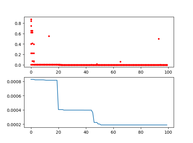
-> Demo code: [examples/demo_ga.py#s3](https://github.com/guofei9987/scikit-opt/blob/master/examples/demo_ga.py#L22)
```python
import pandas as pd
import matplotlib.pyplot as plt
Y_history = pd.DataFrame(ga.all_history_Y)
fig, ax = plt.subplots(2, 1)
ax[0].plot(Y_history.index, Y_history.values, '.', color='red')
Y_history.min(axis=1).cummin().plot(kind='line')
plt.show()
```
### 2.2 Genetic Algorithm for TSP(Travelling Salesman Problem)
Just import the `GA_TSP`, it overloads the `crossover`, `mutation` to solve the TSP
**Step1**: define your problem. Prepare your points coordinate and the distance matrix.
Here I generate the data randomly as a demo:
-> Demo code: [examples/demo_ga_tsp.py#s1](https://github.com/guofei9987/scikit-opt/blob/master/examples/demo_ga_tsp.py#L1)
```python
import numpy as np
from scipy import spatial
import matplotlib.pyplot as plt
num_points = 50
points_coordinate = np.random.rand(num_points, 2) # generate coordinate of points
distance_matrix = spatial.distance.cdist(points_coordinate, points_coordinate, metric='euclidean')
def cal_total_distance(routine):
'''The objective function. input routine, return total distance.
cal_total_distance(np.arange(num_points))
'''
num_points, = routine.shape
return sum([distance_matrix[routine[i % num_points], routine[(i + 1) % num_points]] for i in range(num_points)])
```
**Step2**: do GA
-> Demo code: [examples/demo_ga_tsp.py#s2](https://github.com/guofei9987/scikit-opt/blob/master/examples/demo_ga_tsp.py#L19)
```python
from sko.GA import GA_TSP
ga_tsp = GA_TSP(func=cal_total_distance, n_dim=num_points, size_pop=50, max_iter=500, prob_mut=1)
best_points, best_distance = ga_tsp.run()
```
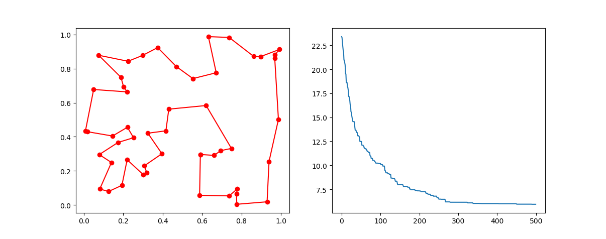
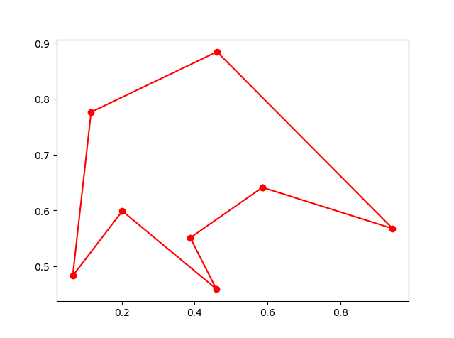
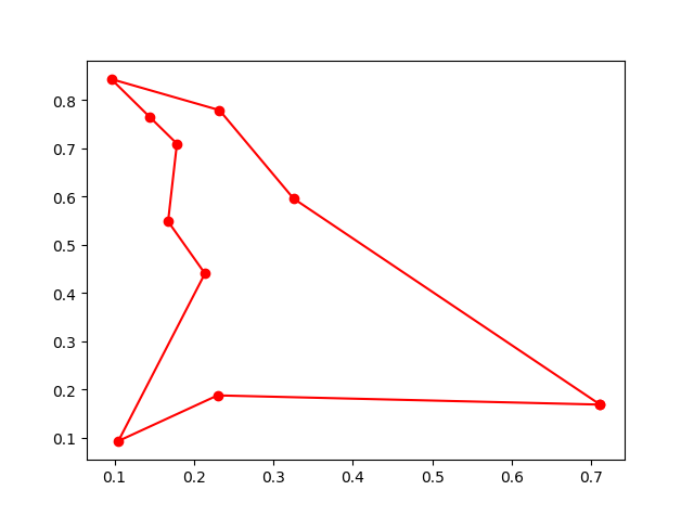
**Step3**: Plot the result:
-> Demo code: [examples/demo_ga_tsp.py#s3](https://github.com/guofei9987/scikit-opt/blob/master/examples/demo_ga_tsp.py#L26)
```python
fig, ax = plt.subplots(1, 2)
best_points_ = np.concatenate([best_points, [best_points[0]]])
best_points_coordinate = points_coordinate[best_points_, :]
ax[0].plot(best_points_coordinate[:, 0], best_points_coordinate[:, 1], 'o-r')
ax[1].plot(ga_tsp.generation_best_Y)
plt.show()
```
## 3. PSO(Particle swarm optimization)
### 3.1 PSO
**Step1**: define your problem:
-> Demo code: [examples/demo_pso.py#s1](https://github.com/guofei9987/scikit-opt/blob/master/examples/demo_pso.py#L1)
```python
def demo_func(x):
x1, x2, x3 = x
return x1 ** 2 + (x2 - 0.05) ** 2 + x3 ** 2
```
**Step2**: do PSO
-> Demo code: [examples/demo_pso.py#s2](https://github.com/guofei9987/scikit-opt/blob/master/examples/demo_pso.py#L6)
```python
from sko.PSO import PSO
pso = PSO(func=demo_func, n_dim=3, pop=40, max_iter=150, lb=[0, -1, 0.5], ub=[1, 1, 1], w=0.8, c1=0.5, c2=0.5)
pso.run()
print('best_x is ', pso.gbest_x, 'best_y is', pso.gbest_y)
```
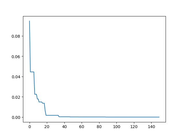
**Step3**: Plot the result
-> Demo code: [examples/demo_pso.py#s3](https://github.com/guofei9987/scikit-opt/blob/master/examples/demo_pso.py#L13)
```python
import matplotlib.pyplot as plt
plt.plot(pso.gbest_y_hist)
plt.show()
```
### 3.2 PSO with nonlinear constraint
If you need nolinear constraint like `(x[0] - 1) ** 2 + (x[1] - 0) ** 2 - 0.5 ** 2<=0`
Codes are like this:
```python
constraint_ueq = (
lambda x: (x[0] - 1) ** 2 + (x[1] - 0) ** 2 - 0.5 ** 2
,
)
pso = PSO(func=demo_func, n_dim=2, pop=40, max_iter=max_iter, lb=[-2, -2], ub=[2, 2]
, constraint_ueq=constraint_ueq)
```
Note that, you can add more then one nonlinear constraint. Just add it to `constraint_ueq`
More over, we have an animation:
↑**see [examples/demo_pso_ani.py](https://github.com/guofei9987/scikit-opt/blob/master/examples/demo_pso_ani.py)**
## 4. SA(Simulated Annealing)
### 4.1 SA for multiple function
**Step1**: define your problem
-> Demo code: [examples/demo_sa.py#s1](https://github.com/guofei9987/scikit-opt/blob/master/examples/demo_sa.py#L1)
```python
demo_func = lambda x: x[0] ** 2 + (x[1] - 0.05) ** 2 + x[2] ** 2
```
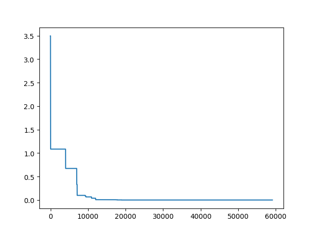
**Step2**: do SA
-> Demo code: [examples/demo_sa.py#s2](https://github.com/guofei9987/scikit-opt/blob/master/examples/demo_sa.py#L3)
```python
from sko.SA import SA
sa = SA(func=demo_func, x0=[1, 1, 1], T_max=1, T_min=1e-9, L=300, max_stay_counter=150)
best_x, best_y = sa.run()
print('best_x:', best_x, 'best_y', best_y)
```
**Step3**: Plot the result
-> Demo code: [examples/demo_sa.py#s3](https://github.com/guofei9987/scikit-opt/blob/master/examples/demo_sa.py#L10)
```python
import matplotlib.pyplot as plt
import pandas as pd
plt.plot(pd.DataFrame(sa.best_y_history).cummin(axis=0))
plt.show()
```
Moreover, scikit-opt provide 3 types of Simulated Annealing: Fast, Boltzmann, Cauchy. See [more sa](https://scikit-opt.github.io/scikit-opt/#/en/more_sa)
### 4.2 SA for TSP
**Step1**: oh, yes, define your problems. To boring to copy this step.
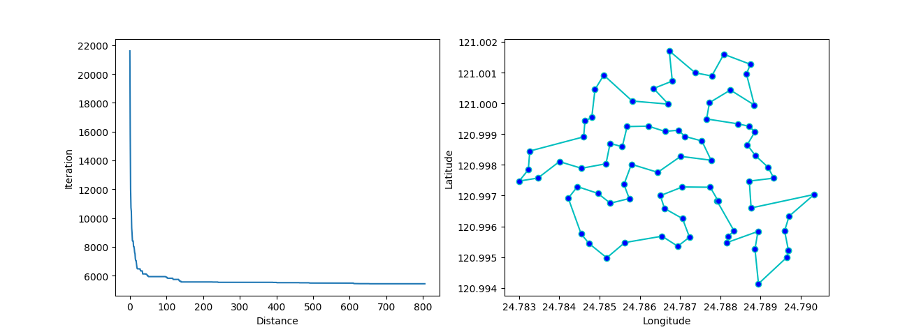
**Step2**: DO SA for TSP
-> Demo code: [examples/demo_sa_tsp.py#s2](https://github.com/guofei9987/scikit-opt/blob/master/examples/demo_sa_tsp.py#L21)
```python
from sko.SA import SA_TSP
sa_tsp = SA_TSP(func=cal_total_distance, x0=range(num_points), T_max=100, T_min=1, L=10 * num_points)
best_points, best_distance = sa_tsp.run()
print(best_points, best_distance, cal_total_distance(best_points))
```
**Step3**: plot the result
-> Demo code: [examples/demo_sa_tsp.py#s3](https://github.com/guofei9987/scikit-opt/blob/master/examples/demo_sa_tsp.py#L28)
```python
from matplotlib.ticker import FormatStrFormatter
fig, ax = plt.subplots(1, 2)
best_points_ = np.concatenate([best_points, [best_points[0]]])
best_points_coordinate = points_coordinate[best_points_, :]
ax[0].plot(sa_tsp.best_y_history)
ax[0].set_xlabel("Iteration")
ax[0].set_ylabel("Distance")
ax[1].plot(best_points_coordinate[:, 0], best_points_coordinate[:, 1],
marker='o', markerfacecolor='b', color='c', linestyle='-')
ax[1].xaxis.set_major_formatter(FormatStrFormatter('%.3f'))
ax[1].yaxis.set_major_formatter(FormatStrFormatter('%.3f'))
ax[1].set_xlabel("Longitude")
ax[1].set_ylabel("Latitude")
plt.show()
```
More: Plot the animation:
↑**see [examples/demo_sa_tsp.py](https://github.com/guofei9987/scikit-opt/blob/master/examples/demo_sa_tsp.py)**
## 5. ACA (Ant Colony Algorithm) for tsp
-> Demo code: [examples/demo_aca_tsp.py#s2](https://github.com/guofei9987/scikit-opt/blob/master/examples/demo_aca_tsp.py#L17)
```python
from sko.ACA import ACA_TSP
aca = ACA_TSP(func=cal_total_distance, n_dim=num_points,
size_pop=50, max_iter=200,
distance_matrix=distance_matrix)
best_x, best_y = aca.run()
```
## 6. immune algorithm (IA)
-> Demo code: [examples/demo_ia.py#s2](https://github.com/guofei9987/scikit-opt/blob/master/examples/demo_ia.py#L6)
```python
from sko.IA import IA_TSP
ia_tsp = IA_TSP(func=cal_total_distance, n_dim=num_points, size_pop=500, max_iter=800, prob_mut=0.2,
T=0.7, alpha=0.95)
best_points, best_distance = ia_tsp.run()
print('best routine:', best_points, 'best_distance:', best_distance)
```
## 7. Artificial Fish Swarm Algorithm (AFSA)
-> Demo code: [examples/demo_afsa.py#s1](https://github.com/guofei9987/scikit-opt/blob/master/examples/demo_afsa.py#L1)
```python
def func(x):
x1, x2 = x
return 1 / x1 ** 2 + x1 ** 2 + 1 / x2 ** 2 + x2 ** 2
from sko.AFSA import AFSA
afsa = AFSA(func, n_dim=2, size_pop=50, max_iter=300,
max_try_num=100, step=0.5, visual=0.3,
q=0.98, delta=0.5)
best_x, best_y = afsa.run()
print(best_x, best_y)
```
# Projects using scikit-opt
- [Yu, J., He, Y., Yan, Q., & Kang, X. (2021). SpecView: Malware Spectrum Visualization Framework With Singular Spectrum Transformation. IEEE Transactions on Information Forensics and Security, 16, 5093-5107.](https://ieeexplore.ieee.org/abstract/document/9607026/)
- [Zhen, H., Zhai, H., Ma, W., Zhao, L., Weng, Y., Xu, Y., ... & He, X. (2021). Design and tests of reinforcement-learning-based optimal power flow solution generator. Energy Reports.](https://www.sciencedirect.com/science/article/pii/S2352484721012737)
- [Heinrich, K., Zschech, P., Janiesch, C., & Bonin, M. (2021). Process data properties matter: Introducing gated convolutional neural networks (GCNN) and key-value-predict attention networks (KVP) for next event prediction with deep learning. Decision Support Systems, 143, 113494.](https://www.sciencedirect.com/science/article/pii/S016792362100004X)
- [Tang, H. K., & Goh, S. K. (2021). A Novel Non-population-based Meta-heuristic Optimizer Inspired by the Philosophy of Yi Jing. arXiv preprint arXiv:2104.08564.](https://arxiv.org/abs/2104.08564)
- [Wu, G., Li, L., Li, X., Chen, Y., Chen, Z., Qiao, B., ... & Xia, L. (2021). Graph embedding based real-time social event matching for EBSNs recommendation. World Wide Web, 1-22.](https://link.springer.com/article/10.1007/s11280-021-00934-y)
- [Pan, X., Zhang, Z., Zhang, H., Wen, Z., Ye, W., Yang, Y., ... & Zhao, X. (2021). A fast and robust mixture gases identification and concentration detection algorithm based on attention mechanism equipped recurrent neural network with double loss function. Sensors and Actuators B: Chemical, 342, 129982.](https://www.sciencedirect.com/science/article/abs/pii/S0925400521005517)
- [Castella Balcell, M. (2021). Optimization of the station keeping system for the WindCrete floating offshore wind turbine.](https://upcommons.upc.edu/handle/2117/350262)
- [Zhai, B., Wang, Y., Wang, W., & Wu, B. (2021). Optimal Variable Speed Limit Control Strategy on Freeway Segments under Fog Conditions. arXiv preprint arXiv:2107.14406.](https://arxiv.org/abs/2107.14406)
- [Yap, X. H. (2021). Multi-label classification on locally-linear data: Application to chemical toxicity prediction.](https://etd.ohiolink.edu/apexprod/rws_olink/r/1501/10?clear=10&p10_accession_num=wright162901936395651)
- [Gebhard, L. (2021). Expansion Planning of Low-Voltage Grids Using Ant Colony Optimization Ausbauplanung von Niederspannungsnetzen mithilfe eines Ameisenalgorithmus.](https://ad-publications.cs.uni-freiburg.de/theses/Master_Lukas_Gebhard_2021.pdf)
- [Ma, X., Zhou, H., & Li, Z. (2021). Optimal Design for Interdependencies between Hydrogen and Power Systems. IEEE Transactions on Industry Applications.](https://ieeexplore.ieee.org/abstract/document/9585654)
- [de Curso, T. D. C. (2021). Estudo do modelo Johansen-Ledoit-Sornette de bolhas financeiras.](https://d1wqtxts1xzle7.cloudfront.net/67649721/TCC_Thibor_Final-with-cover-page-v2.pdf?Expires=1639140872&Signature=LDZoVsAGO0mLMlVsQjnzpLlRhLyt5wdIDmBjm1yWog5bsx6apyRE9aHuwfnFnc96uvam573wiHMeV08QlK2vhRcQS1d0buenBT5fwoRuq6PTDoMsXmpBb-lGtu9ETiMb4sBYvcQb-X3C7Hh0Ec1FoJZ040gXJPWdAli3e1TdOcGrnOaBZMgNiYX6aKFIZaaXmiQeV3418~870bH4IOQXOapIE6-23lcOL-32T~FSjsOrENoLUkcosv6UHPourKgsRufAY-C2HBUWP36iJ7CoH0jSTo1e45dVgvqNDvsHz7tmeI~0UPGH-A8MWzQ9h2ElCbCN~UNQ8ycxOa4TUKfpCw__&Key-Pair-Id=APKAJLOHF5GGSLRBV4ZA)
- [Wu, T., Liu, J., Liu, J., Huang, Z., Wu, H., Zhang, C., ... & Zhang, G. (2021). A Novel AI-based Framework for AoI-optimal Trajectory Planning in UAV-assisted Wireless Sensor Networks. IEEE Transactions on Wireless Communications.](https://ieeexplore.ieee.org/abstract/document/9543607)
- [Liu, H., Wen, Z., & Cai, W. (2021, August). FastPSO: Towards Efficient Swarm Intelligence Algorithm on GPUs. In 50th International Conference on Parallel Processing (pp. 1-10).](https://dl.acm.org/doi/abs/10.1145/3472456.3472474)
- [Mahbub, R. (2020). Algorithms and Optimization Techniques for Solving TSP.](https://raiyanmahbub.com/images/Research_Paper.pdf)
- [Li, J., Chen, T., Lim, K., Chen, L., Khan, S. A., Xie, J., & Wang, X. (2019). Deep learning accelerated gold nanocluster synthesis. Advanced Intelligent Systems, 1(3), 1900029.](https://onlinelibrary.wiley.com/doi/full/10.1002/aisy.201900029)
Raw data
{
"_id": null,
"home_page": "https://github.com/guofei9987/scikit-opt",
"name": "scikit-opt",
"maintainer": "",
"docs_url": null,
"requires_python": ">=3.5",
"maintainer_email": "",
"keywords": "",
"author": "Guo Fei",
"author_email": "guofei9987@foxmail.com",
"download_url": "https://files.pythonhosted.org/packages/59/63/eb0c1c56d7de607cdf93f3ba96e8c631f2da2e734ec32fd7a667fb8594a9/scikit-opt-0.6.6.tar.gz",
"platform": "linux",
"description": "\n\n# [scikit-opt](https://github.com/guofei9987/scikit-opt)\n\n[](https://pypi.org/project/scikit-opt/)\n[](https://travis-ci.com/guofei9987/scikit-opt)\n[](https://codecov.io/gh/guofei9987/scikit-opt)\n[](https://github.com/guofei9987/scikit-opt/blob/master/LICENSE)\n\n\n[](https://github.com/guofei9987/scikit-opt/fork)\n[](https://pepy.tech/project/scikit-opt)\n[](https://github.com/guofei9987/scikit-opt/discussions)\n\n\n\n\nSwarm Intelligence in Python \n(Genetic Algorithm, Particle Swarm Optimization, Simulated Annealing, Ant Colony Algorithm, Immune Algorithm,Artificial Fish Swarm Algorithm in Python) \n\n\n- **Documentation:** [https://scikit-opt.github.io/scikit-opt/#/en/](https://scikit-opt.github.io/scikit-opt/#/en/)\n- **\u6587\u6863\uff1a** [https://scikit-opt.github.io/scikit-opt/#/zh/](https://scikit-opt.github.io/scikit-opt/#/zh/) \n- **Source code:** [https://github.com/guofei9987/scikit-opt](https://github.com/guofei9987/scikit-opt)\n- **Help us improve scikit-opt** [https://www.wjx.cn/jq/50964691.aspx](https://www.wjx.cn/jq/50964691.aspx)\n\n# install\n```bash\npip install scikit-opt\n```\n\nFor the current developer version:\n```bach\ngit clone git@github.com:guofei9987/scikit-opt.git\ncd scikit-opt\npip install .\n```\n\n# Features\n## Feature1: UDF\n\n**UDF** (user defined function) is available now!\n\nFor example, you just worked out a new type of `selection` function. \nNow, your `selection` function is like this: \n-> Demo code: [examples/demo_ga_udf.py#s1](https://github.com/guofei9987/scikit-opt/blob/master/examples/demo_ga_udf.py#L1)\n```python\n# step1: define your own operator:\ndef selection_tournament(algorithm, tourn_size):\n FitV = algorithm.FitV\n sel_index = []\n for i in range(algorithm.size_pop):\n aspirants_index = np.random.choice(range(algorithm.size_pop), size=tourn_size)\n sel_index.append(max(aspirants_index, key=lambda i: FitV[i]))\n algorithm.Chrom = algorithm.Chrom[sel_index, :] # next generation\n return algorithm.Chrom\n\n\n```\n\nImport and build ga \n-> Demo code: [examples/demo_ga_udf.py#s2](https://github.com/guofei9987/scikit-opt/blob/master/examples/demo_ga_udf.py#L12)\n```python\nimport numpy as np\nfrom sko.GA import GA, GA_TSP\n\ndemo_func = lambda x: x[0] ** 2 + (x[1] - 0.05) ** 2 + (x[2] - 0.5) ** 2\nga = GA(func=demo_func, n_dim=3, size_pop=100, max_iter=500, prob_mut=0.001,\n lb=[-1, -10, -5], ub=[2, 10, 2], precision=[1e-7, 1e-7, 1])\n\n```\nRegist your udf to GA \n-> Demo code: [examples/demo_ga_udf.py#s3](https://github.com/guofei9987/scikit-opt/blob/master/examples/demo_ga_udf.py#L20)\n```python\nga.register(operator_name='selection', operator=selection_tournament, tourn_size=3)\n```\n\nscikit-opt also provide some operators \n-> Demo code: [examples/demo_ga_udf.py#s4](https://github.com/guofei9987/scikit-opt/blob/master/examples/demo_ga_udf.py#L22)\n```python\nfrom sko.operators import ranking, selection, crossover, mutation\n\nga.register(operator_name='ranking', operator=ranking.ranking). \\\n register(operator_name='crossover', operator=crossover.crossover_2point). \\\n register(operator_name='mutation', operator=mutation.mutation)\n```\nNow do GA as usual \n-> Demo code: [examples/demo_ga_udf.py#s5](https://github.com/guofei9987/scikit-opt/blob/master/examples/demo_ga_udf.py#L28)\n```python\nbest_x, best_y = ga.run()\nprint('best_x:', best_x, '\\n', 'best_y:', best_y)\n```\n\n> Until Now, the **udf** surport `crossover`, `mutation`, `selection`, `ranking` of GA\n> scikit-opt provide a dozen of operators, see [here](https://github.com/guofei9987/scikit-opt/tree/master/sko/operators)\n\nFor advanced users:\n\n-> Demo code: [examples/demo_ga_udf.py#s6](https://github.com/guofei9987/scikit-opt/blob/master/examples/demo_ga_udf.py#L31)\n```python\nclass MyGA(GA):\n def selection(self, tourn_size=3):\n FitV = self.FitV\n sel_index = []\n for i in range(self.size_pop):\n aspirants_index = np.random.choice(range(self.size_pop), size=tourn_size)\n sel_index.append(max(aspirants_index, key=lambda i: FitV[i]))\n self.Chrom = self.Chrom[sel_index, :] # next generation\n return self.Chrom\n\n ranking = ranking.ranking\n\n\ndemo_func = lambda x: x[0] ** 2 + (x[1] - 0.05) ** 2 + (x[2] - 0.5) ** 2\nmy_ga = MyGA(func=demo_func, n_dim=3, size_pop=100, max_iter=500, lb=[-1, -10, -5], ub=[2, 10, 2],\n precision=[1e-7, 1e-7, 1])\nbest_x, best_y = my_ga.run()\nprint('best_x:', best_x, '\\n', 'best_y:', best_y)\n```\n\n## feature2: continue to run\n(New in version 0.3.6) \nRun an algorithm for 10 iterations, and then run another 20 iterations base on the 10 iterations before:\n```python\nfrom sko.GA import GA\n\nfunc = lambda x: x[0] ** 2\nga = GA(func=func, n_dim=1)\nga.run(10)\nga.run(20)\n```\n\n## feature3: 4-ways to accelerate\n- vectorization\n- multithreading\n- multiprocessing\n- cached\n\nsee [https://github.com/guofei9987/scikit-opt/blob/master/examples/example_function_modes.py](https://github.com/guofei9987/scikit-opt/blob/master/examples/example_function_modes.py)\n\n\n\n## feature4: GPU computation\n We are developing GPU computation, which will be stable on version 1.0.0 \nAn example is already available: [https://github.com/guofei9987/scikit-opt/blob/master/examples/demo_ga_gpu.py](https://github.com/guofei9987/scikit-opt/blob/master/examples/demo_ga_gpu.py)\n\n\n# Quick start\n\n## 1. Differential Evolution\n**Step1**\uff1adefine your problem \n-> Demo code: [examples/demo_de.py#s1](https://github.com/guofei9987/scikit-opt/blob/master/examples/demo_de.py#L1)\n```python\n'''\nmin f(x1, x2, x3) = x1^2 + x2^2 + x3^2\ns.t.\n x1*x2 >= 1\n x1*x2 <= 5\n x2 + x3 = 1\n 0 <= x1, x2, x3 <= 5\n'''\n\n\ndef obj_func(p):\n x1, x2, x3 = p\n return x1 ** 2 + x2 ** 2 + x3 ** 2\n\n\nconstraint_eq = [\n lambda x: 1 - x[1] - x[2]\n]\n\nconstraint_ueq = [\n lambda x: 1 - x[0] * x[1],\n lambda x: x[0] * x[1] - 5\n]\n\n```\n\n**Step2**: do Differential Evolution \n-> Demo code: [examples/demo_de.py#s2](https://github.com/guofei9987/scikit-opt/blob/master/examples/demo_de.py#L25)\n```python\nfrom sko.DE import DE\n\nde = DE(func=obj_func, n_dim=3, size_pop=50, max_iter=800, lb=[0, 0, 0], ub=[5, 5, 5],\n constraint_eq=constraint_eq, constraint_ueq=constraint_ueq)\n\nbest_x, best_y = de.run()\nprint('best_x:', best_x, '\\n', 'best_y:', best_y)\n\n```\n\n## 2. Genetic Algorithm\n\n**Step1**\uff1adefine your problem \n-> Demo code: [examples/demo_ga.py#s1](https://github.com/guofei9987/scikit-opt/blob/master/examples/demo_ga.py#L1)\n```python\nimport numpy as np\n\n\ndef schaffer(p):\n '''\n This function has plenty of local minimum, with strong shocks\n global minimum at (0,0) with value 0\n https://en.wikipedia.org/wiki/Test_functions_for_optimization\n '''\n x1, x2 = p\n part1 = np.square(x1) - np.square(x2)\n part2 = np.square(x1) + np.square(x2)\n return 0.5 + (np.square(np.sin(part1)) - 0.5) / np.square(1 + 0.001 * part2)\n\n\n```\n\n**Step2**: do Genetic Algorithm \n-> Demo code: [examples/demo_ga.py#s2](https://github.com/guofei9987/scikit-opt/blob/master/examples/demo_ga.py#L16)\n```python\nfrom sko.GA import GA\n\nga = GA(func=schaffer, n_dim=2, size_pop=50, max_iter=800, prob_mut=0.001, lb=[-1, -1], ub=[1, 1], precision=1e-7)\nbest_x, best_y = ga.run()\nprint('best_x:', best_x, '\\n', 'best_y:', best_y)\n```\n\n-> Demo code: [examples/demo_ga.py#s3](https://github.com/guofei9987/scikit-opt/blob/master/examples/demo_ga.py#L22)\n```python\nimport pandas as pd\nimport matplotlib.pyplot as plt\n\nY_history = pd.DataFrame(ga.all_history_Y)\nfig, ax = plt.subplots(2, 1)\nax[0].plot(Y_history.index, Y_history.values, '.', color='red')\nY_history.min(axis=1).cummin().plot(kind='line')\nplt.show()\n```\n\n\n\n### 2.2 Genetic Algorithm for TSP(Travelling Salesman Problem)\nJust import the `GA_TSP`, it overloads the `crossover`, `mutation` to solve the TSP\n\n**Step1**: define your problem. Prepare your points coordinate and the distance matrix. \nHere I generate the data randomly as a demo: \n-> Demo code: [examples/demo_ga_tsp.py#s1](https://github.com/guofei9987/scikit-opt/blob/master/examples/demo_ga_tsp.py#L1)\n```python\nimport numpy as np\nfrom scipy import spatial\nimport matplotlib.pyplot as plt\n\nnum_points = 50\n\npoints_coordinate = np.random.rand(num_points, 2) # generate coordinate of points\ndistance_matrix = spatial.distance.cdist(points_coordinate, points_coordinate, metric='euclidean')\n\n\ndef cal_total_distance(routine):\n '''The objective function. input routine, return total distance.\n cal_total_distance(np.arange(num_points))\n '''\n num_points, = routine.shape\n return sum([distance_matrix[routine[i % num_points], routine[(i + 1) % num_points]] for i in range(num_points)])\n\n\n```\n\n**Step2**: do GA \n-> Demo code: [examples/demo_ga_tsp.py#s2](https://github.com/guofei9987/scikit-opt/blob/master/examples/demo_ga_tsp.py#L19)\n```python\n\nfrom sko.GA import GA_TSP\n\nga_tsp = GA_TSP(func=cal_total_distance, n_dim=num_points, size_pop=50, max_iter=500, prob_mut=1)\nbest_points, best_distance = ga_tsp.run()\n\n```\n\n**Step3**: Plot the result: \n-> Demo code: [examples/demo_ga_tsp.py#s3](https://github.com/guofei9987/scikit-opt/blob/master/examples/demo_ga_tsp.py#L26)\n```python\nfig, ax = plt.subplots(1, 2)\nbest_points_ = np.concatenate([best_points, [best_points[0]]])\nbest_points_coordinate = points_coordinate[best_points_, :]\nax[0].plot(best_points_coordinate[:, 0], best_points_coordinate[:, 1], 'o-r')\nax[1].plot(ga_tsp.generation_best_Y)\nplt.show()\n```\n\n\n\n\n## 3. PSO(Particle swarm optimization)\n\n### 3.1 PSO\n**Step1**: define your problem: \n-> Demo code: [examples/demo_pso.py#s1](https://github.com/guofei9987/scikit-opt/blob/master/examples/demo_pso.py#L1)\n```python\ndef demo_func(x):\n x1, x2, x3 = x\n return x1 ** 2 + (x2 - 0.05) ** 2 + x3 ** 2\n\n\n```\n\n**Step2**: do PSO \n-> Demo code: [examples/demo_pso.py#s2](https://github.com/guofei9987/scikit-opt/blob/master/examples/demo_pso.py#L6)\n```python\nfrom sko.PSO import PSO\n\npso = PSO(func=demo_func, n_dim=3, pop=40, max_iter=150, lb=[0, -1, 0.5], ub=[1, 1, 1], w=0.8, c1=0.5, c2=0.5)\npso.run()\nprint('best_x is ', pso.gbest_x, 'best_y is', pso.gbest_y)\n\n```\n\n**Step3**: Plot the result \n-> Demo code: [examples/demo_pso.py#s3](https://github.com/guofei9987/scikit-opt/blob/master/examples/demo_pso.py#L13)\n```python\nimport matplotlib.pyplot as plt\n\nplt.plot(pso.gbest_y_hist)\nplt.show()\n```\n\n\n\n\n### 3.2 PSO with nonlinear constraint\n\nIf you need nolinear constraint like `(x[0] - 1) ** 2 + (x[1] - 0) ** 2 - 0.5 ** 2<=0` \nCodes are like this:\n```python\nconstraint_ueq = (\n lambda x: (x[0] - 1) ** 2 + (x[1] - 0) ** 2 - 0.5 ** 2\n ,\n)\npso = PSO(func=demo_func, n_dim=2, pop=40, max_iter=max_iter, lb=[-2, -2], ub=[2, 2]\n , constraint_ueq=constraint_ueq)\n```\n\nNote that, you can add more then one nonlinear constraint. Just add it to `constraint_ueq`\n\nMore over, we have an animation: \n \n\u2191**see [examples/demo_pso_ani.py](https://github.com/guofei9987/scikit-opt/blob/master/examples/demo_pso_ani.py)**\n\n\n## 4. SA(Simulated Annealing)\n### 4.1 SA for multiple function\n**Step1**: define your problem \n-> Demo code: [examples/demo_sa.py#s1](https://github.com/guofei9987/scikit-opt/blob/master/examples/demo_sa.py#L1)\n```python\ndemo_func = lambda x: x[0] ** 2 + (x[1] - 0.05) ** 2 + x[2] ** 2\n\n```\n**Step2**: do SA \n-> Demo code: [examples/demo_sa.py#s2](https://github.com/guofei9987/scikit-opt/blob/master/examples/demo_sa.py#L3)\n```python\nfrom sko.SA import SA\n\nsa = SA(func=demo_func, x0=[1, 1, 1], T_max=1, T_min=1e-9, L=300, max_stay_counter=150)\nbest_x, best_y = sa.run()\nprint('best_x:', best_x, 'best_y', best_y)\n\n```\n\n**Step3**: Plot the result \n-> Demo code: [examples/demo_sa.py#s3](https://github.com/guofei9987/scikit-opt/blob/master/examples/demo_sa.py#L10)\n```python\nimport matplotlib.pyplot as plt\nimport pandas as pd\n\nplt.plot(pd.DataFrame(sa.best_y_history).cummin(axis=0))\nplt.show()\n\n```\n\n\n\nMoreover, scikit-opt provide 3 types of Simulated Annealing: Fast, Boltzmann, Cauchy. See [more sa](https://scikit-opt.github.io/scikit-opt/#/en/more_sa)\n### 4.2 SA for TSP\n**Step1**: oh, yes, define your problems. To boring to copy this step. \n\n**Step2**: DO SA for TSP \n-> Demo code: [examples/demo_sa_tsp.py#s2](https://github.com/guofei9987/scikit-opt/blob/master/examples/demo_sa_tsp.py#L21)\n```python\nfrom sko.SA import SA_TSP\n\nsa_tsp = SA_TSP(func=cal_total_distance, x0=range(num_points), T_max=100, T_min=1, L=10 * num_points)\n\nbest_points, best_distance = sa_tsp.run()\nprint(best_points, best_distance, cal_total_distance(best_points))\n```\n\n**Step3**: plot the result \n-> Demo code: [examples/demo_sa_tsp.py#s3](https://github.com/guofei9987/scikit-opt/blob/master/examples/demo_sa_tsp.py#L28)\n```python\nfrom matplotlib.ticker import FormatStrFormatter\n\nfig, ax = plt.subplots(1, 2)\n\nbest_points_ = np.concatenate([best_points, [best_points[0]]])\nbest_points_coordinate = points_coordinate[best_points_, :]\nax[0].plot(sa_tsp.best_y_history)\nax[0].set_xlabel(\"Iteration\")\nax[0].set_ylabel(\"Distance\")\nax[1].plot(best_points_coordinate[:, 0], best_points_coordinate[:, 1],\n marker='o', markerfacecolor='b', color='c', linestyle='-')\nax[1].xaxis.set_major_formatter(FormatStrFormatter('%.3f'))\nax[1].yaxis.set_major_formatter(FormatStrFormatter('%.3f'))\nax[1].set_xlabel(\"Longitude\")\nax[1].set_ylabel(\"Latitude\")\nplt.show()\n\n```\n\n\n\nMore: Plot the animation: \n\n \n\u2191**see [examples/demo_sa_tsp.py](https://github.com/guofei9987/scikit-opt/blob/master/examples/demo_sa_tsp.py)**\n\n\n\n\n## 5. ACA (Ant Colony Algorithm) for tsp\n-> Demo code: [examples/demo_aca_tsp.py#s2](https://github.com/guofei9987/scikit-opt/blob/master/examples/demo_aca_tsp.py#L17)\n```python\nfrom sko.ACA import ACA_TSP\n\naca = ACA_TSP(func=cal_total_distance, n_dim=num_points,\n size_pop=50, max_iter=200,\n distance_matrix=distance_matrix)\n\nbest_x, best_y = aca.run()\n\n```\n\n\n\n\n## 6. immune algorithm (IA)\n-> Demo code: [examples/demo_ia.py#s2](https://github.com/guofei9987/scikit-opt/blob/master/examples/demo_ia.py#L6)\n```python\n\nfrom sko.IA import IA_TSP\n\nia_tsp = IA_TSP(func=cal_total_distance, n_dim=num_points, size_pop=500, max_iter=800, prob_mut=0.2,\n T=0.7, alpha=0.95)\nbest_points, best_distance = ia_tsp.run()\nprint('best routine:', best_points, 'best_distance:', best_distance)\n\n```\n\n\n\n## 7. Artificial Fish Swarm Algorithm (AFSA)\n-> Demo code: [examples/demo_afsa.py#s1](https://github.com/guofei9987/scikit-opt/blob/master/examples/demo_afsa.py#L1)\n```python\ndef func(x):\n x1, x2 = x\n return 1 / x1 ** 2 + x1 ** 2 + 1 / x2 ** 2 + x2 ** 2\n\n\nfrom sko.AFSA import AFSA\n\nafsa = AFSA(func, n_dim=2, size_pop=50, max_iter=300,\n max_try_num=100, step=0.5, visual=0.3,\n q=0.98, delta=0.5)\nbest_x, best_y = afsa.run()\nprint(best_x, best_y)\n```\n\n\n# Projects using scikit-opt\n\n- [Yu, J., He, Y., Yan, Q., & Kang, X. (2021). SpecView: Malware Spectrum Visualization Framework With Singular Spectrum Transformation. IEEE Transactions on Information Forensics and Security, 16, 5093-5107.](https://ieeexplore.ieee.org/abstract/document/9607026/)\n- [Zhen, H., Zhai, H., Ma, W., Zhao, L., Weng, Y., Xu, Y., ... & He, X. (2021). Design and tests of reinforcement-learning-based optimal power flow solution generator. Energy Reports.](https://www.sciencedirect.com/science/article/pii/S2352484721012737)\n- [Heinrich, K., Zschech, P., Janiesch, C., & Bonin, M. (2021). Process data properties matter: Introducing gated convolutional neural networks (GCNN) and key-value-predict attention networks (KVP) for next event prediction with deep learning. Decision Support Systems, 143, 113494.](https://www.sciencedirect.com/science/article/pii/S016792362100004X)\n- [Tang, H. K., & Goh, S. K. (2021). A Novel Non-population-based Meta-heuristic Optimizer Inspired by the Philosophy of Yi Jing. arXiv preprint arXiv:2104.08564.](https://arxiv.org/abs/2104.08564)\n- [Wu, G., Li, L., Li, X., Chen, Y., Chen, Z., Qiao, B., ... & Xia, L. (2021). Graph embedding based real-time social event matching for EBSNs recommendation. World Wide Web, 1-22.](https://link.springer.com/article/10.1007/s11280-021-00934-y)\n- [Pan, X., Zhang, Z., Zhang, H., Wen, Z., Ye, W., Yang, Y., ... & Zhao, X. (2021). A fast and robust mixture gases identification and concentration detection algorithm based on attention mechanism equipped recurrent neural network with double loss function. Sensors and Actuators B: Chemical, 342, 129982.](https://www.sciencedirect.com/science/article/abs/pii/S0925400521005517)\n- [Castella Balcell, M. (2021). Optimization of the station keeping system for the WindCrete floating offshore wind turbine.](https://upcommons.upc.edu/handle/2117/350262)\n- [Zhai, B., Wang, Y., Wang, W., & Wu, B. (2021). Optimal Variable Speed Limit Control Strategy on Freeway Segments under Fog Conditions. arXiv preprint arXiv:2107.14406.](https://arxiv.org/abs/2107.14406)\n- [Yap, X. H. (2021). Multi-label classification on locally-linear data: Application to chemical toxicity prediction.](https://etd.ohiolink.edu/apexprod/rws_olink/r/1501/10?clear=10&p10_accession_num=wright162901936395651)\n- [Gebhard, L. (2021). Expansion Planning of Low-Voltage Grids Using Ant Colony Optimization Ausbauplanung von Niederspannungsnetzen mithilfe eines Ameisenalgorithmus.](https://ad-publications.cs.uni-freiburg.de/theses/Master_Lukas_Gebhard_2021.pdf)\n- [Ma, X., Zhou, H., & Li, Z. (2021). Optimal Design for Interdependencies between Hydrogen and Power Systems. IEEE Transactions on Industry Applications.](https://ieeexplore.ieee.org/abstract/document/9585654)\n- [de Curso, T. D. C. (2021). Estudo do modelo Johansen-Ledoit-Sornette de bolhas financeiras.](https://d1wqtxts1xzle7.cloudfront.net/67649721/TCC_Thibor_Final-with-cover-page-v2.pdf?Expires=1639140872&Signature=LDZoVsAGO0mLMlVsQjnzpLlRhLyt5wdIDmBjm1yWog5bsx6apyRE9aHuwfnFnc96uvam573wiHMeV08QlK2vhRcQS1d0buenBT5fwoRuq6PTDoMsXmpBb-lGtu9ETiMb4sBYvcQb-X3C7Hh0Ec1FoJZ040gXJPWdAli3e1TdOcGrnOaBZMgNiYX6aKFIZaaXmiQeV3418~870bH4IOQXOapIE6-23lcOL-32T~FSjsOrENoLUkcosv6UHPourKgsRufAY-C2HBUWP36iJ7CoH0jSTo1e45dVgvqNDvsHz7tmeI~0UPGH-A8MWzQ9h2ElCbCN~UNQ8ycxOa4TUKfpCw__&Key-Pair-Id=APKAJLOHF5GGSLRBV4ZA)\n- [Wu, T., Liu, J., Liu, J., Huang, Z., Wu, H., Zhang, C., ... & Zhang, G. (2021). A Novel AI-based Framework for AoI-optimal Trajectory Planning in UAV-assisted Wireless Sensor Networks. IEEE Transactions on Wireless Communications.](https://ieeexplore.ieee.org/abstract/document/9543607)\n- [Liu, H., Wen, Z., & Cai, W. (2021, August). FastPSO: Towards Efficient Swarm Intelligence Algorithm on GPUs. In 50th International Conference on Parallel Processing (pp. 1-10).](https://dl.acm.org/doi/abs/10.1145/3472456.3472474)\n- [Mahbub, R. (2020). Algorithms and Optimization Techniques for Solving TSP.](https://raiyanmahbub.com/images/Research_Paper.pdf)\n- [Li, J., Chen, T., Lim, K., Chen, L., Khan, S. A., Xie, J., & Wang, X. (2019). Deep learning accelerated gold nanocluster synthesis. Advanced Intelligent Systems, 1(3), 1900029.](https://onlinelibrary.wiley.com/doi/full/10.1002/aisy.201900029)\n\n\n",
"bugtrack_url": null,
"license": "MIT",
"summary": "Swarm Intelligence in Python",
"version": "0.6.6",
"split_keywords": [],
"urls": [
{
"comment_text": "",
"digests": {
"md5": "0b753fca0593ec836218020c0aa74e36",
"sha256": "dd83d33d6748a0c8d4962c241493875f7e1b39eeea17251c6b1f94d5bff79069"
},
"downloads": -1,
"filename": "scikit_opt-0.6.6-py3-none-any.whl",
"has_sig": false,
"md5_digest": "0b753fca0593ec836218020c0aa74e36",
"packagetype": "bdist_wheel",
"python_version": "py3",
"requires_python": ">=3.5",
"size": 35079,
"upload_time": "2022-01-14T08:49:08",
"upload_time_iso_8601": "2022-01-14T08:49:08.015592Z",
"url": "https://files.pythonhosted.org/packages/57/b6/a35676427b36636e4a408f1dca346b30b803ed278e91887465366e41fcf2/scikit_opt-0.6.6-py3-none-any.whl",
"yanked": false,
"yanked_reason": null
},
{
"comment_text": "",
"digests": {
"md5": "8575064094d238ee341cf1da39f2aaef",
"sha256": "3e620789d16a0552f0893497be81c53f75171cfcf0aec0b43a051fa9df8f9879"
},
"downloads": -1,
"filename": "scikit-opt-0.6.6.tar.gz",
"has_sig": false,
"md5_digest": "8575064094d238ee341cf1da39f2aaef",
"packagetype": "sdist",
"python_version": "source",
"requires_python": ">=3.5",
"size": 41720,
"upload_time": "2022-01-14T08:49:10",
"upload_time_iso_8601": "2022-01-14T08:49:10.840468Z",
"url": "https://files.pythonhosted.org/packages/59/63/eb0c1c56d7de607cdf93f3ba96e8c631f2da2e734ec32fd7a667fb8594a9/scikit-opt-0.6.6.tar.gz",
"yanked": false,
"yanked_reason": null
}
],
"upload_time": "2022-01-14 08:49:10",
"github": true,
"gitlab": false,
"bitbucket": false,
"github_user": "guofei9987",
"github_project": "scikit-opt",
"travis_ci": true,
"coveralls": false,
"github_actions": false,
"requirements": [
{
"name": "numpy",
"specs": []
},
{
"name": "scipy",
"specs": []
},
{
"name": "matplotlib",
"specs": []
},
{
"name": "pandas",
"specs": []
}
],
"lcname": "scikit-opt"
}


